Low-Level Parent Phase Reconstruction

This page rebuilds the triple-point workflow from Triple-Point-Based Parent Phase Reconstruction with low-level functions. It exposes the candidate variant IDs, vote counts, grain-ID remapping, and per-pixel parent calculation that the parentGrainReconstructor normally manages.

Use this route when you need to inspect or replace one of those operations. For a routine reconstruction, the higher-level workflow is shorter and less vulnerable to inconsistent bookkeeping.

import numpy as np

from mtex import *

ebsd = mtexdata('alphaBetaTitanium', verbose=False)

alphaName = 'Ti (alpha)'
betaName = 'Ti (Beta)'

plot(ebsd[alphaName], ebsd[alphaName].orientations, figSize='large')

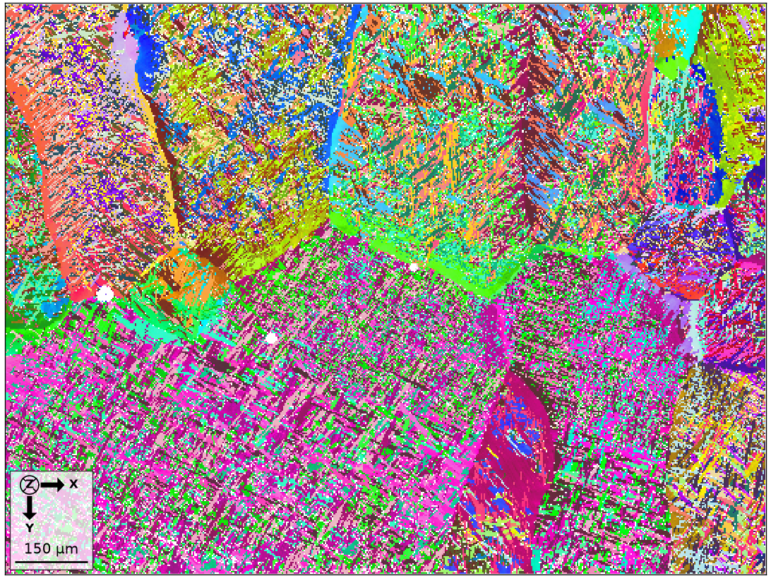
The preceding page measures the same 99.8% alpha and 0.2% beta phase fractions and explains what to notice in this map. It also defines the Burgers OR and the required parent-to-child direction. We reuse that OR without redefining it here.

beta2alpha = orientation.Burgers(ebsd[betaName].CS, ebsd[alphaName].CS)
beta2alpha

misorientation (Ti (BETA) → Ti (alpha))
  (110) || (0001)   [1̅11̅] || [21̅1̅0]

Segment grains for triple-point analysis

The preceding page defines a triple point and explains why this workflow uses a 1.5-degree segmentation threshold with removeQuadruplePoints. We add one boundary-smoothing iteration while keeping the triple points attached to the boundary network.

grains = calcGrains(ebsd, threshold=1.5 * degree, removeQuadruplePoints=True)
grains = smoothBoundary(grains, 1, moveTriplePoints=True)

region = [299, 401, 440, 500]
plot(ebsd[alphaName], ebsd[alphaName].orientations, region=region, micronbar='off', figSize='large')

hold(True)
plot(grains.boundary, lineWidth=2, region=region)
hold(False)

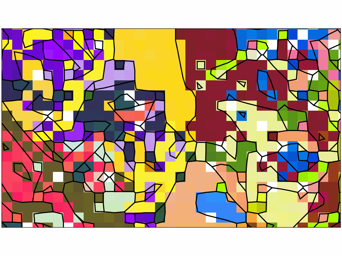
The black lines show how finely the 1.5-degree threshold partitions the alpha map. Each former four-way junction is now a pair of three-segment junctions. Smoothing has turned the network into free-form polygons, so those pairs are not something to pick out by eye here; the next step counts them instead.

Compute two parent candidates at every triple point

Extract only alpha-alpha-alpha triple points. The high-level calcTPVotes call performed this phase selection internally.

tP = grains.triplePoints(alphaName, alphaName, alphaName)
tP

triplePointList (y↓→x)
  size: 85338
  points   mineral 1   mineral 2   mineral 3
   85338  Ti (alpha)  Ti (alpha)  Ti (alpha)

calcParent tests the three mean alpha orientations at each point against all Burgers variants. The id flag returns variant IDs instead of parent orientations. The numFit=2 option retains the best and second-best combinations.

tPori = grains.selectByGrainId(tP.grainId).meanOrientation.reshape(-1, 3)
tripleParentId, tripleFit = calcParent(tPori, beta2alpha, numFit=2, id=True, threshold=5 * degree)

tripleFitQuantiles = np.nanquantile(tripleFit[:, 0] / degree, [0.25, 0.5, 0.75])
print(tripleFitQuantiles)

hold(True)
plot(tP, tripleFit[:, 0] / degree, markerEdgeColor='k', markerSize=10, region=region)
setColorRange([0, 5])
mtexColorMap('LaboTeX')
mtexColorbar(title='best fit (degrees)')
hold(False)

[1.1562 1.5311 2.0373]

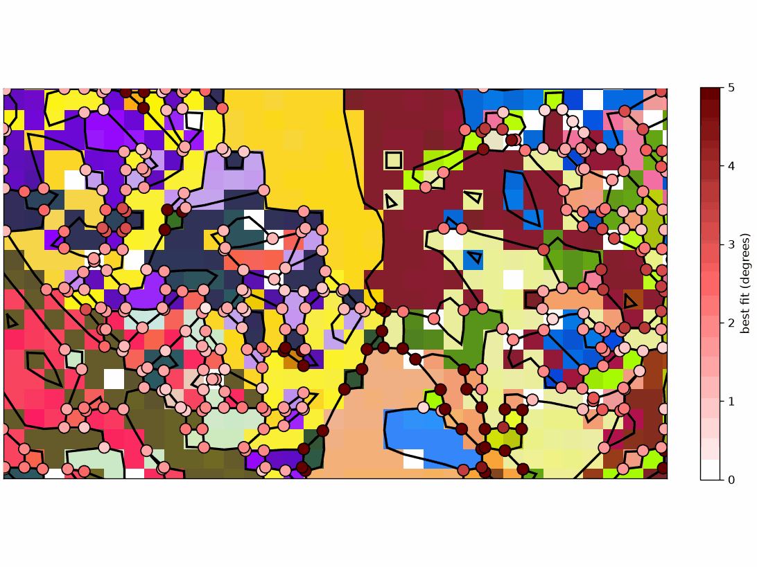
The first fit is the largest pairwise mismatch among the three candidate parent orientations, reported in radians by calcParent and converted to degrees here. Its quartiles are 1.156, 1.531, and 2.038 degrees. The colour map runs from white at zero to dark red at five degrees, so the palest markers are the triples compatible with one beta orientation and the dark ones are the misfits the next section rejects.

Reject ambiguous triple points

Keep a triple point when its best fit is below 2.5 degrees and its second-best fit is above 2.5 degrees. This low-level example uses the same value on both sides of the decision. The preceding high-level page imposed a wider ambiguity gap by requiring its second-best fit to exceed 5 degrees.

consistentTP = (tripleFit[:, 0] < 2.5 * degree) & (tripleFit[:, 1] > 2.5 * degree)
numConsistentTriplePoints = np.count_nonzero(consistentTP)
print(numConsistentTriplePoints)

hold(True)
plot(tP[consistentTP], markerEdgeColor='r', markerSize=10, markerFaceColor='none', lineWidth=2, region=region)
hold(False)

54824

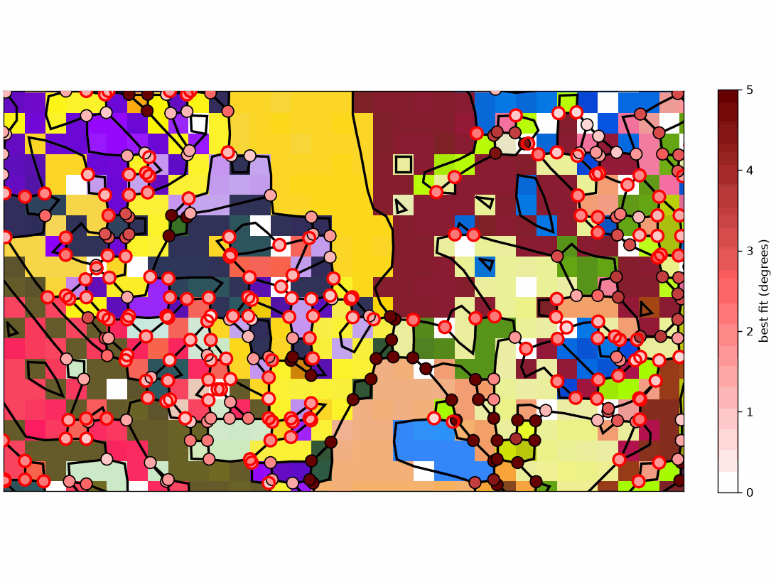
Red circles mark 54,868 retained seeds. Many survive even though the best-fit cutoff is sharp. The next check asks whether a grain receives compatible variant IDs from all of its retained triple points.

Require consistent votes within each child grain

Each retained triple point casts one variant-ID vote for each of its three grains. majorityVote with strict returns an ID only when every vote received by that grain is identical. Conflicting grains receive NaN.

seedParentId, numVotes = majorityVote(tP[consistentTP].grainId, tripleParentId[consistentTP, 0, :], grains.id.max(), strict=True)

numVotes is the number of agreeing triple-point votes, not the number of unique IDs. Requiring numVotes > 2 therefore means at least three votes.

hasSeed = numVotes > 2
numSeedGrains = np.count_nonzero(hasSeed)
print(numSeedGrains)

parentGrains = grains.copy()
parentGrains[hasSeed] = variants(beta2alpha, grains[hasSeed].meanOrientation, seedParentId[hasSeed].astype(int))

ipfKey = ipfColorKey(ebsd[betaName])
ipfKey.ipfDirection = vector3d.Y

parentColor = ipfKey.orientation2color(parentGrains[betaName].meanOrientation)
plot(parentGrains[betaName], parentColor, figSize='large')

26804

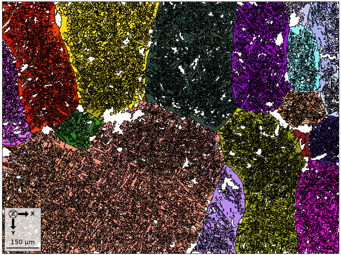
The vote requirement transforms 26,828 child grains into coloured beta fragments. Their footprints still follow the original alpha boundaries because no merge has occurred.

Reject isolated seeds before merging

As an additional consistency check, require every proposed parent component to contain at least two measured child grains. A test run of merge returns the proposed old-to-new grain IDs without modifying the map.

trialMergeId = parentGrains.merge(threshold=2.5 * degree, testRun=True)
trialComponentSize = np.bincount(trialMergeId)

setBack = (trialComponentSize[trialMergeId] < 2) & hasSeed
numIsolatedSeeds = np.count_nonzero(setBack)
print(numIsolatedSeeds)

parentGrains[setBack] = grains[setBack].meanOrientation

10

Only the seeded grains can be set back, so hasSeed restricts the test to them. This check reverts the 9 seeds that would have stood alone and leaves 26,819 of the 26,828 in place. It can be omitted when independent single-grain parents are plausible.

Merge the accepted seed fragments

Neighbouring beta fragments within 2.5 degrees are now merged. seedMergeId, the parentId the merge writes, maps every original grain to its current grain ID.

merged = parentGrains.merge(threshold=2.5 * degree)
seedMergeId = parentGrains.parentId
parentGrains = merged
numSeedParentGrains = len(parentGrains[betaName])
numSeedParentGrains

113

The EBSD map needs the same ID change. A connected notIndexed area can be a grain, so all pixels must be remapped rather than only indexed pixels. The leading zero preserves pixels whose grain ID is zero.

parentEBSD = ebsd.copy()
old2new = np.r_[0, seedMergeId]
parentEBSD.grainId = old2new[ebsd.grainId]

parentColor = ipfKey.orientation2color(parentGrains[betaName].meanOrientation)
plot(parentGrains[betaName], parentColor, figSize='large')

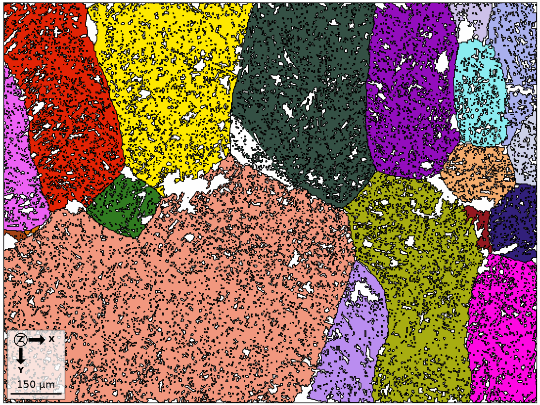
Compatible fragments now form 114 beta-grain footprints. Remaining alpha grains are candidates for growth from a reconstructed neighbour.

Find alpha grains next to reconstructed beta grains

neighbors returns the IDs of neighbouring alpha and beta grains. For every pair, calcParent compares the measured alpha orientation with the reconstructed beta orientation.

grainPairs = parentGrains[alphaName].neighbors(parentGrains[betaName])

oriAlpha = parentGrains.selectByGrainId(grainPairs[:, 0]).meanOrientation
oriBeta = parentGrains.selectByGrainId(grainPairs[:, 1]).meanOrientation

pairParentId, pairFit = calcParent(oriAlpha, oriBeta, beta2alpha, numFit=2, id=True)

pairFitQuantiles = np.nanquantile(pairFit[:, 0] / degree, [0.25, 0.5, 0.75])
pairFitQuantiles

array([0.9663, 1.4263, 2.129 ])

The first returned ID selects the alpha variant compatible with its beta neighbour. Its fit quartiles are 0.966, 1.427, and 2.129 degrees. The second fit exposes whether that choice is unambiguous.

Transform alpha grains supported by boundary pairs

The executable criterion keeps pairs whose best fit is below 5 degrees and whose second-best fit is above 5 degrees. Earlier prose and its threshold summary called this a 2.5-degree step, but that did not match the code.

consistentPairs = (pairFit[:, 0] < 5 * degree) & (pairFit[:, 1] > 5 * degree)
numConsistentPairs = np.count_nonzero(consistentPairs)
numConsistentPairs

16261

Here majorityVote is used without strict. An alpha grain with conflicting neighbours therefore takes its most frequent candidate rather than being rejected outright.

growthParentId, _ = majorityVote(grainPairs[consistentPairs, 0], pairParentId[consistentPairs, 0], parentGrains.id.max())

hasGrowthVote = ~np.isnan(growthParentId)
numGrownAlphaGrains = np.count_nonzero(hasGrowthVote)
print(numGrownAlphaGrains)

parentGrains[hasGrowthVote] = variants(beta2alpha, parentGrains[hasGrowthVote].meanOrientation, growthParentId[hasGrowthVote].astype(int))

merged = parentGrains.merge(threshold=5 * degree)
growthMergeId = parentGrains.parentId
parentGrains = merged

old2new = np.r_[0, growthMergeId]
parentEBSD.grainId = old2new[parentEBSD.grainId]

remainingAlphaPercent = 100 * parentGrains[alphaName].numPixel.sum() / parentGrains.numPixel.sum()
print(remainingAlphaPercent)

parentColor = ipfKey.orientation2color(parentGrains[betaName].meanOrientation)
plot(parentGrains[betaName], parentColor, lineWidth=2, figSize='large')

16216
1.229701864421342

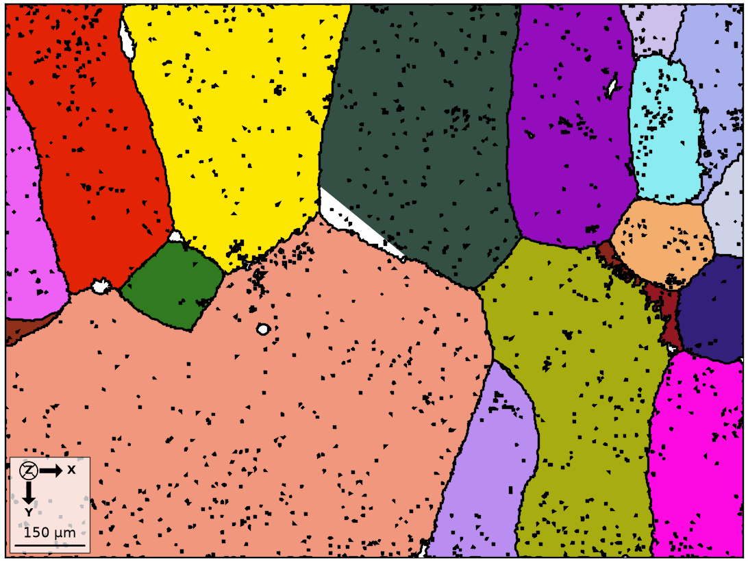
Of 16,251 consistent pairs, the majority vote transforms 16,205 alpha grains. The unreconstructed alpha area is then 1.207%. Repeating the pair-vote step with gradually increasing thresholds can grow the reconstruction further, but each relaxation also accepts weaker fits.

The original page also proposed treating the remaining alpha grains as noise and replacing them during denoising. The closing denoising step below fills only sites with missing orientations; indexed alpha pixels remain alpha unless they are first removed from the map.

Reconstruct a beta orientation at each transformed pixel

The grain means are beta orientations, but the EBSD pixels still store their measured alpha orientations. Select original alpha pixels whose remapped grain now has the beta phase; the grain ids and the phases are read as flat arrays over the gridded map.

gid = parentEBSD.grainId.reshape(-1)
isNowBeta = (parentGrains.phaseId[np.maximum(1, gid) - 1] == ebsd.name2id(betaName)) & \
            (parentEBSD.phaseId.reshape(-1) == ebsd.name2id(alphaName))

With a measured child orientation and a reconstructed parent grain, calcParent returns the compatible beta orientation and its angular fit.

parentOri, pixelFit = calcParent(parentEBSD[isNowBeta].orientations, parentGrains.selectByGrainId(gid[isNowBeta]).meanOrientation,
                                 beta2alpha)
parentEBSD[isNowBeta] = parentOri

pixelFitQuantiles = np.nanquantile(pixelFit / degree, [0.5, 0.9, 0.99])
print(pixelFitQuantiles)

plot(parentEBSD[isNowBeta], pixelFit / degree, figSize='large')
mtexColorbar(title='fit (degrees)')
setColorRange([0, 5])
mtexColorMap('LaboTeX')

hold(True)
plot(parentGrains.boundary, lineWidth=2)
hold(False)

[1.1843 2.0883 3.2105]

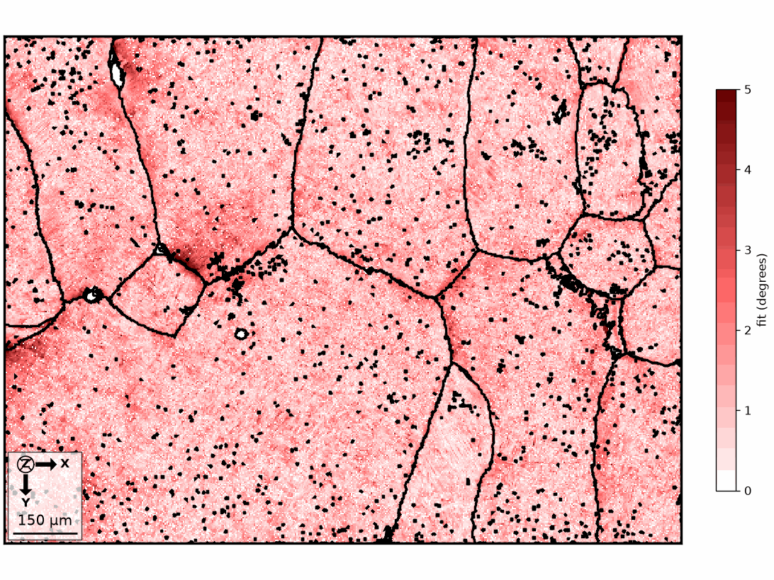
The median pixel fit is 1.183 degrees, 90% are below 2.087 degrees, and 99% are below 3.209 degrees. Low values indicate agreement with the Burgers variant predicted by the beta grain. The boundary overlay shows whether high fits concentrate near reconstructed grain edges.

parentColor = ipfKey.orientation2color(parentEBSD[betaName].orientations)
plot(parentEBSD[betaName], parentColor, figSize='large')

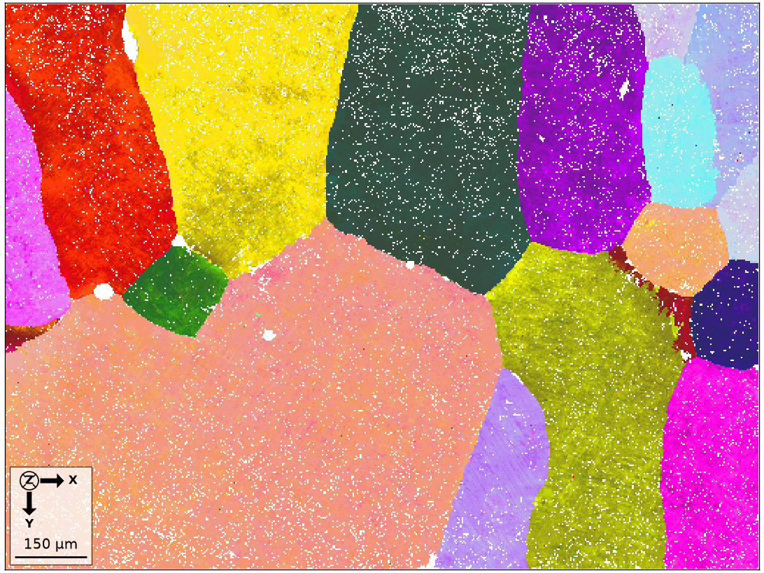
The beta pixel map follows the merged parent footprints while preserving intra-grain orientation variation that was absent from the grain-mean map.

Denoise the reconstructed beta phase

Segment the current parent map at 5 degrees and mark indexed grains smaller than 15 pixels as notIndexed. Five smoothing iterations regularize the retained boundaries.

parentGrains = calcGrains(parentEBSD, angle=5 * degree, minPixel=15)
parentGrains = smoothBoundary(parentGrains, 5)

A halfQuadraticFilter with a small alpha preserves more local detail. The fill option interpolates missing orientations inside the supplied grain boundaries.

F = halfQuadraticFilter()
F.alpha = 0.1
parentEBSD = smooth(parentEBSD, F, fill=parentGrains)

parentColor = ipfKey.orientation2color(parentEBSD[betaName].orientations)
plot(parentEBSD[betaName], parentColor, figSize='large')

hold(True)
plot(parentGrains.boundary, lineWidth=3)
hold(False)

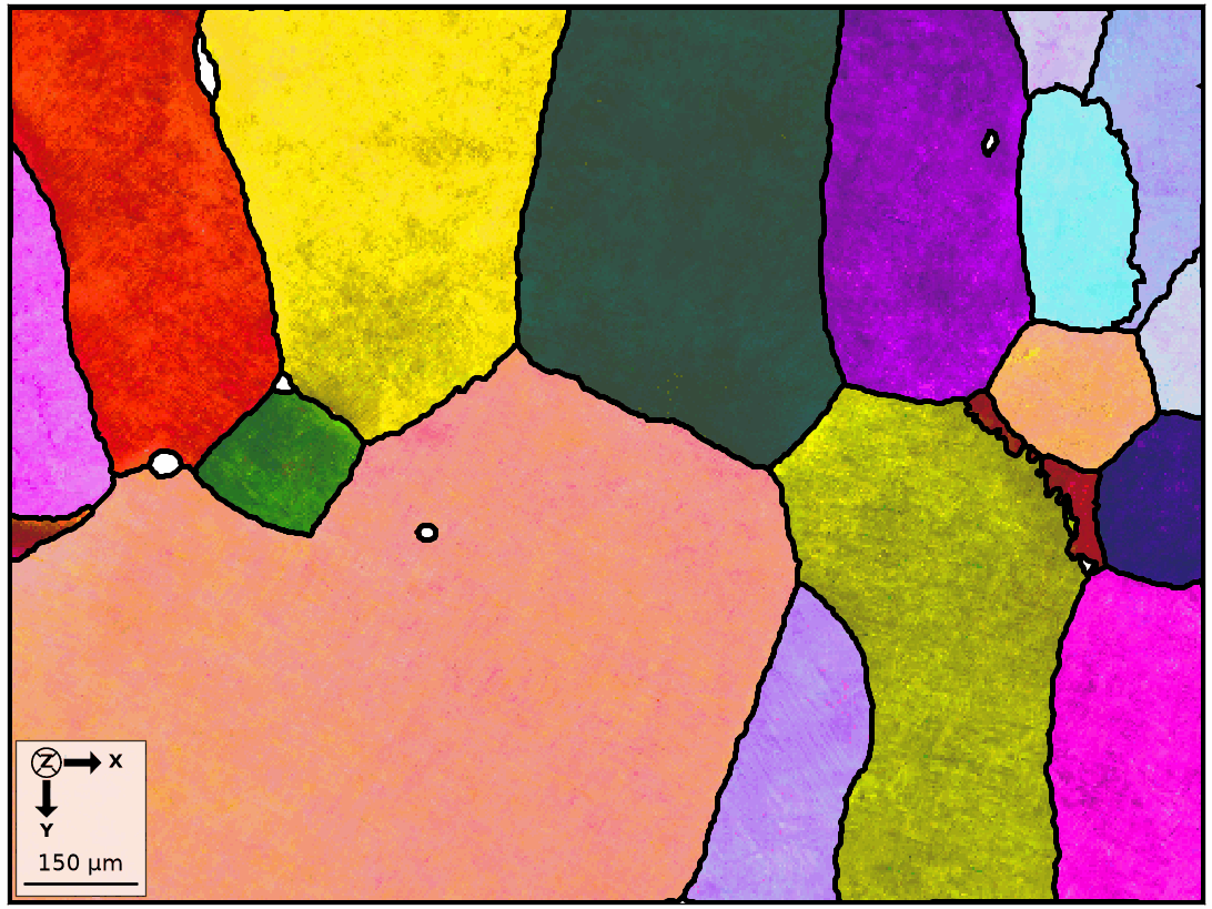
The filter reduces pixel-scale colour variation without blurring across the supplied grain boundaries. It can fill small grains that minPixel changed to notIndexed, but it does not overwrite larger indexed alpha grains.

Compare the final boundaries with the measured child map

Return to the measured alpha orientations and overlay the reconstructed grain boundaries.

plot(ebsd[alphaName], ebsd[alphaName].orientations, figSize='large')
hold(True)
plot(parentGrains.boundary, lineWidth=3, lineColor='white')
hold(False)

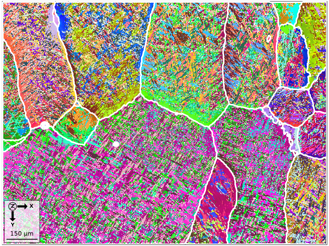
The white outlines should enclose groups of related alpha colours. Boundaries that cut through a visually coherent group are candidates for revisiting the vote or merge thresholds.

Read the intra-grain orientation structure

The final diagnostic colours every beta pixel by the axis and angle of its misorientation from the mean orientation of its grain.

betaPixels = parentEBSD[betaName]
betaMean = parentGrains.selectByGrainId(betaPixels.grainId.reshape(-1)).meanOrientation
mis2MeanDegree = angle(betaPixels.orientations.reshape(-1), betaMean) / degree
mis2MeanQuantiles = np.nanquantile(mis2MeanDegree, [0.5, 0.9, 0.99])
print(mis2MeanQuantiles)

cKey = axisAngleColorKey()
deviationColor = cKey.orientation2color(betaPixels.orientations.reshape(-1), betaMean)
plot(betaPixels, deviationColor, figSize='large')

hold(True)
plot(parentGrains.boundary, lineWidth=3)
hold(False)

[1.1632 2.0592 3.1597]

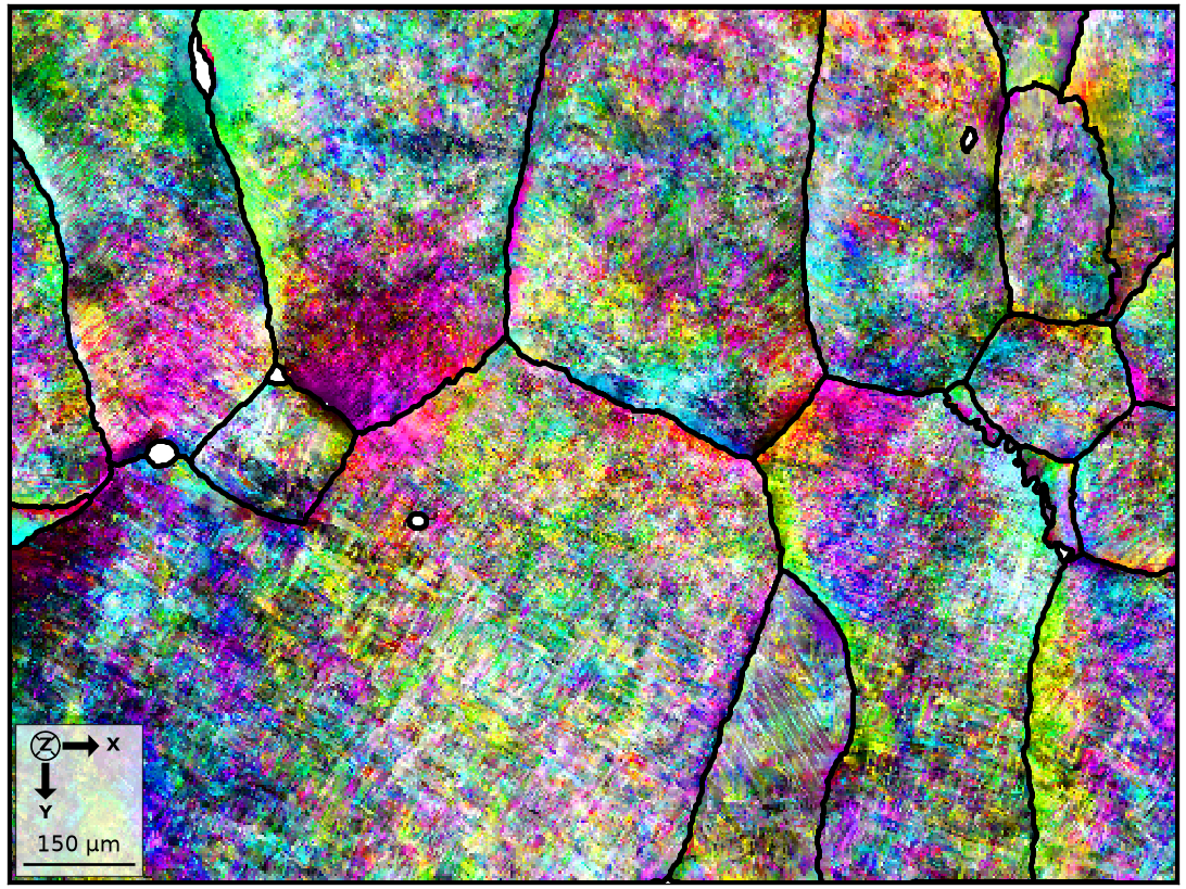
The median deviation from the grain mean is 1.160 degrees, 90% are below 2.054 degrees, and 99% are below 3.147 degrees. Colour changes inside a boundary reveal structure that an IPF map of grain means would hide. Large coherent deviations can indicate deformation or an over-merged grain.

Thresholds used on this page

• Initial child-grain segmentation: 1.5 degrees.
• Best triple-point fit: below 2.5 degrees.
• Second-best triple-point fit: above 2.5 degrees.
• Strict seed support: at least three agreeing votes.
• Seed-fragment merge: below 2.5 degrees and at least two child grains per proposed parent component. The merge may be skipped if the separate fragments are needed.
• Parent-child pair fit and growth merge: 5 degrees.

The earlier summary listed a minimum of two consistent votes and a 2.5-degree alpha-beta threshold. The executable conditions are three votes and 5 degrees, respectively.

References

• F. Niessen, T. Nyyssönen, A. A. Gazder, and R. Hielscher, Parent grain reconstruction from partially or fully transformed microstructures in MTEX, Journal of Applied Crystallography 55 (2022), 180-194, gives the parent-candidate, voting, transformation, and merging framework implemented manually here.

Next

Continue with Advanced Low-Level Parent Grain Reconstruction to apply low-level candidate fitting and graph clustering to a martensitic steel map.

@article{bachmann2010mtex,
  author  = {F. Bachmann and R. Hielscher and H. Schaeben},
  title   = {Texture Analysis with MTEX - Free and Open Source Software Toolbox},
  journal = {Solid State Phenomena},
  volume  = {160},
  pages   = {63-68},
  year    = {2010},
  doi     = {10.4028/www.scientific.net/SSP.160.63},
  url     = {https://doi.org/10.4028/www.scientific.net/SSP.160.63}
}