Advanced Low-Level Parent Grain Reconstruction

This page reconstructs prior austenite from a martensite EBSD map by constructing similarity matrices directly. It compares two sources of evidence while holding the data and fitted orientation relationship (OR) fixed.

The first matrix scores pairs of neighbouring child grains. The second scores all three child grains meeting at a triple point. The preceding Low-Level Parent Phase Reconstruction explains the manual parent-candidate and grain-ID operations reused here.

import matplotlib.pyplot as plt
import numpy as np
from scipy.sparse import coo_matrix
from scipy.special import erf

from mtex import *

plottingConvention.default('y↑→x')
ebsd = mtexdata('martensite', verbose=False)

Segment the measured martensite

Every indexed measurement in this map is bcc martensite. The phase list carries an empty fcc slot alongside it, and that slot is where the reconstruction writes the austenite it recovers.

csBCC = ebsd.CSList[1]
csFCC = ebsd.CSList[2]

grains = calcGrains(ebsd, angle=3 * degree, minPixel=5, removeQuadruplePoints=True)

plot(ebsd['Iron bcc'], ebsd['Iron bcc'].orientations, figSize='large')
hold(True)
plot(grains.boundary, lineWidth=2)
hold(False)

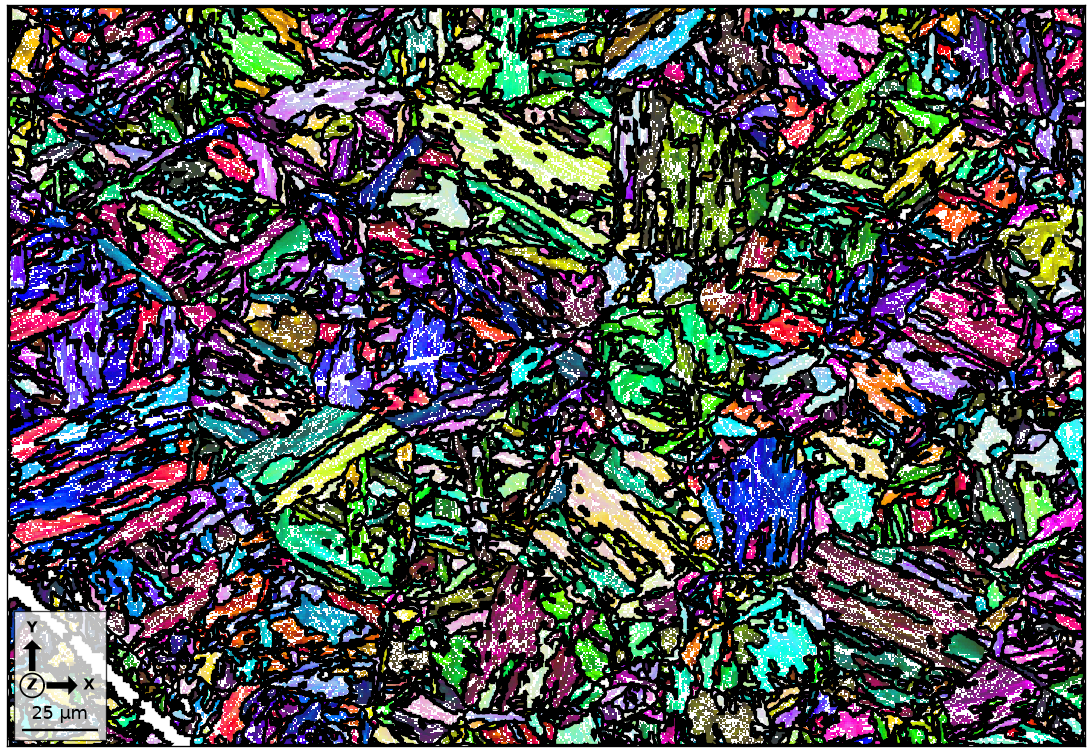
The 3-degree segmentation deliberately divides the martensite into many small child grains. This executable version retains grains of at least five pixels. The earlier version used two pixels, but its two complete low-level graph reconstructions exceeded the page’s practical runtime budget. Black boundaries inside a coherent colour group are candidates to disappear.

Fit the parent-to-child orientation relationship

Parent Austenite Reconstruction explains why the OR must be fitted for each sample. It also introduces the iterative method of Nyyssönen and co-workers. Here the ideal Kurdjumov-Sachs (KS) OR is the initial parent-to-child guess.

KS = orientation.KurdjumovSachs(csFCC, csBCC)

The fit uses a two-column matrix of neighbouring child orientations. Excluding notIndexed grains keeps both columns in the martensite phase. Pairs below 5 degrees are removed because they provide little information about distinct transformation variants.

grainPairs = grains['Iron bcc'].neighbors()
pairOri = grains.selectByGrainId(grainPairs).meanOrientation.reshape(-1, 2)
grainPairs = grainPairs[angle(pairOri[:, 0], pairOri[:, 1]) >= 5 * degree]

fcc2bcc, boundaryFit = calcParent2Child(grains.selectByGrainId(grainPairs).meanOrientation, KS, fit=True)

changeFromKS = angle(KS, fcc2bcc) / degree
print(changeFromKS)
boundaryFitQuantiles = np.nanquantile(boundaryFit / degree, [0.2, 0.4, 0.6, 0.8])
boundaryFitQuantiles

 optimizing parent to child orientation relationship
  scanning 406 orientations
  (347.67°, 10.01°, 56.44°)  2.876
  (347.64°,  9.98°, 56.50°)  2.876
  (347.67°,  9.97°, 56.49°)  2.875
  (347.68°,  9.96°, 56.49°)  2.873
  (347.16°,  9.42°, 57.06°)  2.731
  (347.57°,  9.13°, 56.58°)  2.694
  (347.79°,  9.11°, 56.34°)  2.694
3.424663840367343
array([1.204 , 1.6668, 2.0743, 3.8395])

calcParent2Child assumes that most retained pairs are child-to-child boundaries. It adjusts the OR to reduce their mismatch from theoretical child-to-child misorientations. The fitted OR is 3.132 degrees from KS. Its 20th, 40th, 60th, and 80th fit percentiles are 1.483, 2.018, 2.613, and 4.207 degrees.

plt.close('all')
plt.hist(boundaryFit / degree, bins=50)
plt.xlabel('disorientation angle (degrees)')
plt.ylabel('grain-pair count')

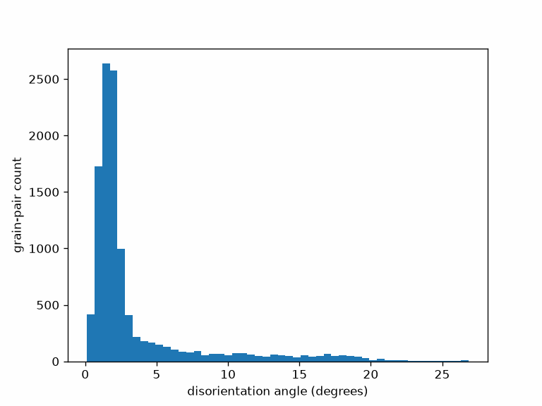
The histogram shows the fitted mismatch distribution. Its low-angle mass supplies the high-similarity relations used by the first clustering route.

Map the boundary evidence

selectByGrainId maps each retained grain pair to all of its boundary segments.

gB, pairId = grains.boundary.selectByGrainId(grainPairs)

plot(ebsd['Iron bcc'], ebsd['Iron bcc'].orientations, figSize='large')
hold(True)
plot(gB, lineWidth=3, lineColor='white')
plot(gB, boundaryFit[pairId] / degree, lineWidth=2)
hold(False)

mtexColorMap('LaboTeX')
mtexColorbar(title='fit (degrees)')
setColorRange([0, 5])

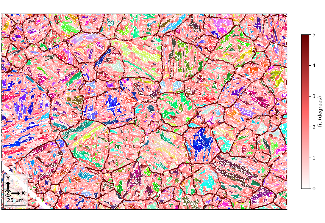
Low-fit segments are compatible with one austenite parent and may become internal boundaries. Large-fit segments join into outlines that are likely to remain as reconstructed parent boundaries.

Convert boundary fit to similarity

A grain graph has one node per grain and an edge for every retained neighbour pair. The edge value below converts angular fit \(\omega\) to the probability-like similarity

The threshold \(t\) is the fit with similarity one half. The tolerance \(s\) controls the transition width. Earlier text called \(s\) the Gaussian standard deviation, but the factor of two in this explicit model means it is not the standard deviation.

omega = np.linspace(0, 5, 100) * degree
boundaryThreshold = 2 * degree
boundaryTolerance = 1.5 * degree

plt.close('all')
plt.plot(omega / degree, 1 - 0.5 * (1 + erf(2 * (omega - boundaryThreshold) / boundaryTolerance)), linewidth=2)
plt.xlabel('fit (degrees)')
plt.ylabel('similarity')

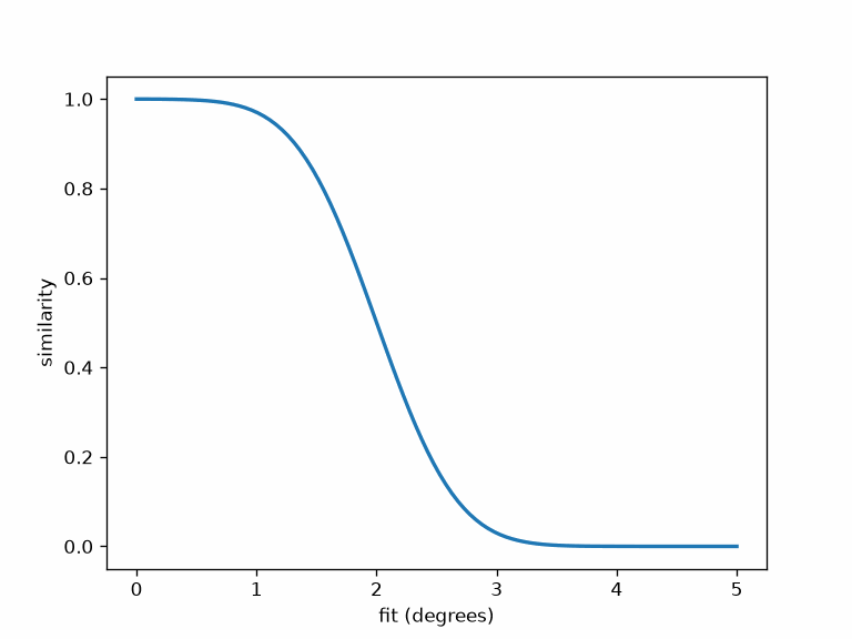
Fits below 2 degrees receive high similarity, while larger fits fall rapidly towards zero. The curve makes the consequences of both parameters visible before they are applied to the map.

boundaryProbability = 1 - 0.5 * (1 + erf(2 * (boundaryFit - boundaryThreshold) / boundaryTolerance))
boundaryProbabilityQuantiles = np.nanquantile(boundaryProbability, [0.1, 0.5, 0.9])
print(boundaryProbabilityQuantiles)

boundaryA = coo_matrix((boundaryProbability, (grainPairs[:, 0] - 1, grainPairs[:, 1] - 1)), shape=(len(grains), len(grains))).tocsr()

[0.     0.5958 0.9797]

The 10th, 50th, and 90th similarity percentiles are 0, 0.3040, and 0.9475. The zero-valued low tail corresponds to badly fitting pairs that should not bind a component.

Cluster the boundary graph

mclComponents applies Markov clustering to the similarity matrix. The inflation power controls cluster granularity. Larger values separate the graph more aggressively.

boundaryInflationPower = 1.6
boundaryA = mclComponents(boundaryA, boundaryInflationPower)

Each resulting component is a candidate parent footprint. merge removes boundaries within a component; grains.parentId is the component of every grain.

boundaryParentGrains = grains.merge(boundaryA)
boundaryParentId = grains.parentId
boundaryParentGrains = smoothBoundary(boundaryParentGrains, 20)
numBoundaryComponents = len(boundaryParentGrains)
numBoundaryComponents

455

All pixels, including pixels in connected notIndexed grains, need the same old-to-new grain-ID mapping. The leading zero preserves pixels that have no grain.

boundaryParentEBSD = ebsd.copy()
old2new = np.r_[0, boundaryParentId]
boundaryParentEBSD.grainId = old2new[ebsd.grainId]

plot(ebsd['Iron bcc'], ebsd['Iron bcc'].orientations, figSize='large')
hold(True)
plot(boundaryParentGrains.boundary, lineWidth=4, lineColor='white')
plot(boundaryParentGrains.boundary, lineWidth=2, lineColor='black')
hold(False)

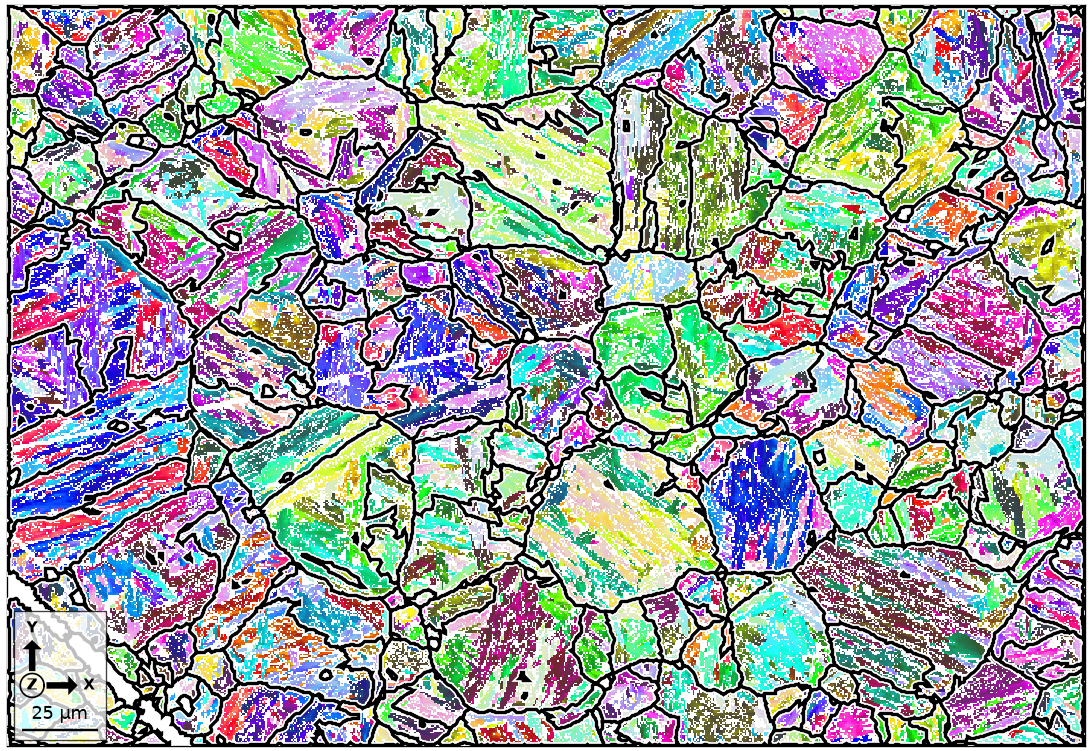
The graph produces 707 candidate components, shown by the double outlines. The components need not have their final size because similarly oriented neighbours can be merged after parent orientations are fitted.

Fit an austenite orientation to every component

calcParent fits one common parent orientation to all martensite grains in a component. Pixel counts weight larger child grains more strongly. Components with fewer than two child grains are left unassigned, and fits of 5 degrees or more are rejected.

childGrains = grains['Iron bcc']
childOri = childGrains.meanOrientation
childComponentId = boundaryParentId[grains.id2ind(childGrains.id)]

componentOri = orientation.nan(boundaryParentId.max(), fcc2bcc.CS)
componentFit = np.full(boundaryParentId.max(), np.inf)
weights = childGrains.numPixel

for k in range(1, boundaryParentId.max() + 1):
  inComponent = childComponentId == k
  if np.count_nonzero(inComponent) > 1:
    componentOri[k - 1], componentFit[k - 1] = calcParent(childOri[inComponent], fcc2bcc, weights=weights[inComponent])

acceptComponent = componentFit < 5 * degree
numAcceptedComponents = np.count_nonzero(acceptComponent)
print(numAcceptedComponents)

boundaryParentGrains[acceptComponent] = componentOri[acceptComponent]

272

Merge similarly oriented parent components

Accepted components have changed from bcc child phase to fcc parent phase. A 4-degree merge combines neighbouring fcc components with similar orientations and returns a second ID mapping. Of the 707 components, 360 pass the child-count and 5-degree fit tests.

numParentsBeforeOrientationMerge = len(boundaryParentGrains['Iron fcc'])
print(numParentsBeforeOrientationMerge)

merged = boundaryParentGrains.merge(threshold=4 * degree)
orientationMergeId = boundaryParentGrains.parentId
boundaryParentGrains = merged

old2new = np.r_[0, orientationMergeId]
boundaryParentEBSD.grainId = old2new[boundaryParentEBSD.grainId]

numParentsAfterOrientationMerge = len(boundaryParentGrains['Iron fcc'])
print(numParentsAfterOrientationMerge)

plot(boundaryParentGrains['Iron fcc'], boundaryParentGrains['Iron fcc'].meanOrientation, figSize='large')

272
162

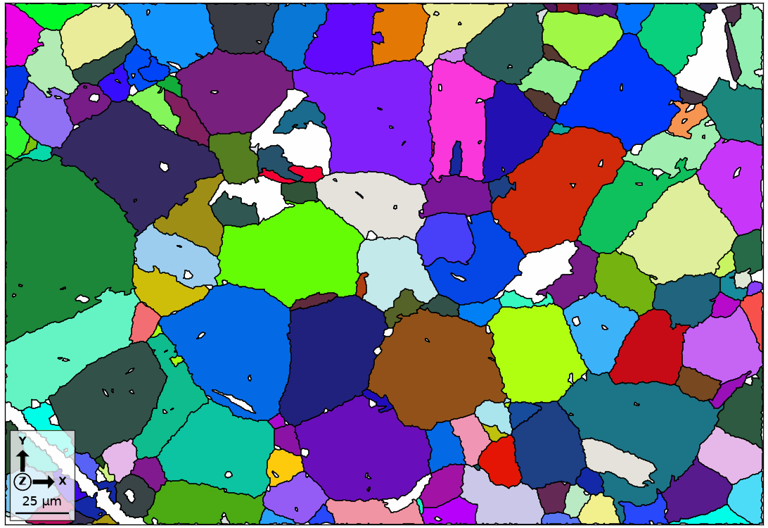
The orientation merge reduces 360 accepted components to 222 fcc parent grains. Their colours identify the reconstructed parent orientations. Neighbours with similar colours have coalesced into larger footprints.

Classify child variants and packets

Parent Austenite Reconstruction defines variants and packets. Here calcVariantId classifies each child against its component orientation. For this OR, packetId selects the parent {111} plane closest to martensite (011).

variantId, packetId, _, _ = calcVariantId(componentOri[childComponentId - 1], childOri, fcc2bcc)

packetColor = ind2color(packetId - 1)
plot(childGrains, packetColor, figSize='large')

hold(True)
plot(boundaryParentGrains.boundary, lineWidth=2)

selectedParentInd = boundaryParentGrains.findByLocation([100, 80])
selectedParent = boundaryParentGrains[selectedParentInd]
selectedParentId = selectedParent.id
print(selectedParentId)
plot(selectedParent.boundary, lineWidth=2, lineColor='white')
hold(False)

[108]

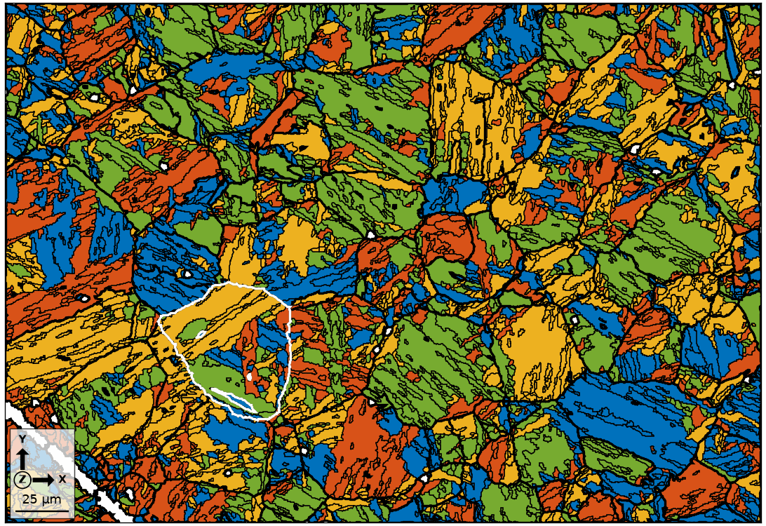
Equal colours identify child grains in the same packet. Black lines show reconstructed parent boundaries, and the white line selects one parent at [100,80]. Earlier prose called it parent 279; this run returns ID 557. The executable lookup avoids assuming that a release-sensitive ID remains fixed.

Check the selected parent’s variants

Plot the measured child poles inside the selected footprint together with poles from the reconstructed parent and all theoretical child variants.

selectedChildOri = ebsd[boundaryParentEBSD.grainId == selectedParentId].orientations
plotPF(selectedChildOri, Miller(0, 0, 1, csBCC), markerSize=3)

hold(True)
selectedParentOri = selectedParent.meanOrientation
plot(selectedParentOri.symmetrise() * Miller(0, 0, 1, csFCC), markerSize=10, marker='s', markerFaceColor='white',
     markerEdgeColor='black', lineWidth=2)

selectedChildVariants = variants(fcc2bcc, selectedParentOri)
plotPF(selectedChildVariants, markerFaceColor='none', lineWidth=2, markerEdgeColor='orange')
hold(False)

  I'm plotting 416 random orientations out of 9358 given orientations
  You can specify the number of points by the option "points".
  The option "all" ensures that all data are plotted

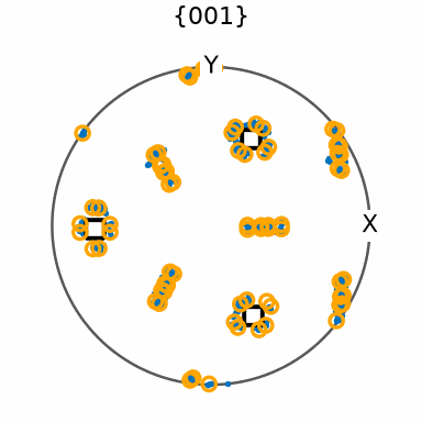
Measured child poles should lie near the orange theoretical variants. Agreement tests the crystallography inside the selected parent rather than only checking its outline.

Reconstruct austenite orientations at individual pixels

Select original martensite pixels whose remapped grain is now fcc; the grain ids and the phases are read as flat arrays over the gridded map.

gid = boundaryParentEBSD.grainId.reshape(-1)
isNowFCC = (boundaryParentGrains.phaseId[np.maximum(1, gid) - 1] == ebsd.name2id('Iron fcc')) & \
           (boundaryParentEBSD.phaseId.reshape(-1) == ebsd.name2id('Iron bcc'))

parentOri, pixelFit = calcParent(ebsd[isNowFCC].orientations, boundaryParentGrains.selectByGrainId(gid[isNowFCC]).meanOrientation, fcc2bcc)
boundaryParentEBSD[isNowFCC] = parentOri

pixelFitQuantiles = np.nanquantile(pixelFit / degree, [0.5, 0.9, 0.99])
print(pixelFitQuantiles)

plot(boundaryParentEBSD['Iron fcc'], boundaryParentEBSD['Iron fcc'].orientations, figSize='large')

[ 1.9241  3.599  10.7584]

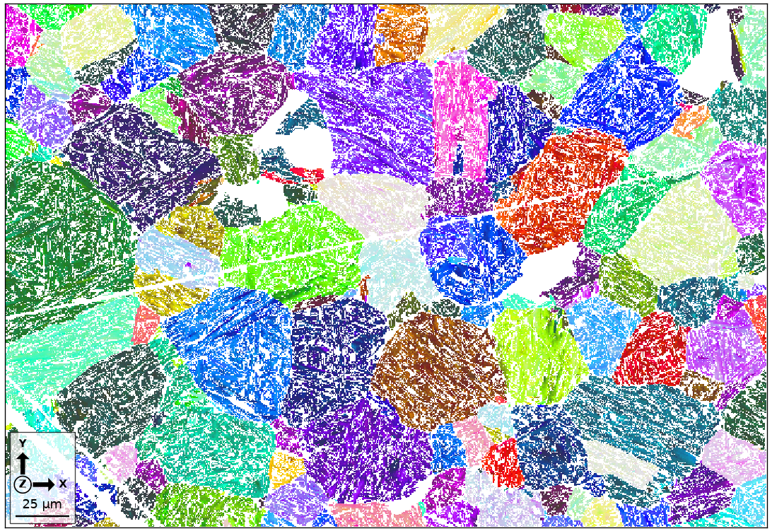
The pixel colours preserve variation inside the reconstructed austenite footprints. Blank regions are not reconstructed as fcc.

plot(boundaryParentEBSD[isNowFCC], pixelFit / degree, figSize='large')
mtexColorMap('LaboTeX')
mtexColorbar(title='fit (degrees)')
setColorRange([0, 5])

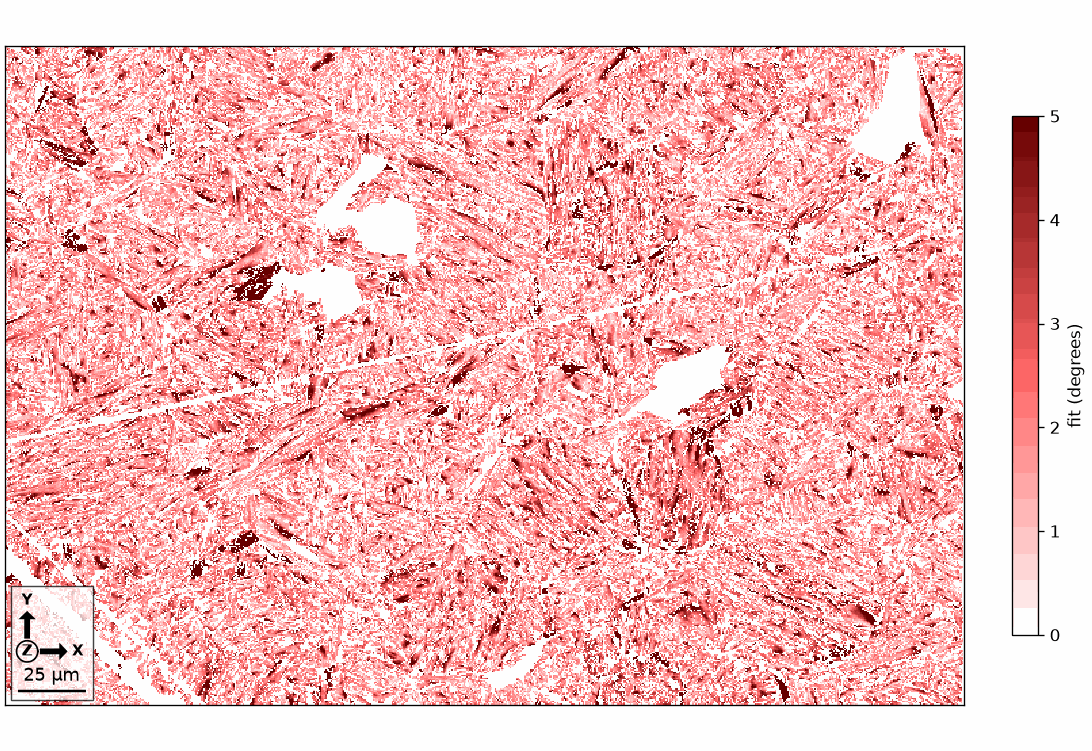
The median pixel fit is 1.830 degrees, 90% are below 3.768 degrees, and 99% are below 10.572 degrees. Low values indicate agreement between a martensite pixel and the variant predicted from its austenite grain.

Denoise and fill missing sites

The preceding Parent Austenite Reconstruction executes the denoising step in full. The same optional sequence for this manually reconstructed map is:

filledEBSD = boundaryParentEBSD['indexed']
filledGrains = calcGrains(filledEBSD, angle=3 * degree, minPixel=10)
filledGrains = smoothBoundary(filledGrains, 20)
F = halfQuadraticFilter()
filledEBSD = smooth(filledEBSD['indexed'], F, fill=filledGrains)
plot(filledEBSD['Iron fcc'], filledEBSD['Iron fcc'].orientations, figSize='large')
hold(True)
plot(filledGrains.boundary, lineWidth=2)
hold(False)

The outlines constrain the fill, so interpolation does not cross the reconstructed boundaries. The filter fills missing and newly removed small-grain sites. Earlier text promised to fill all not reconstructed pixels, but larger indexed bcc regions are not missing and remain bcc.

Boundary-graph thresholds

• Initial child-grain segmentation: 3 degrees and at least five pixels. The earlier page parameter was two pixels; lowering minPixel restores that finer, more expensive child partition.
• Neighbour-pair prefilter: at least 5 degrees.
• Boundary similarity: 2-degree threshold and 1.5-degree tolerance.
• Boundary graph inflation power: 1.6.
• Accepted parent-component fit: below 5 degrees and at least two children.
• Similar-parent merge: below 4 degrees.

Reconstruct footprints from triple points

Boundary evidence can be misleading when child variants from different parents happen to match a theoretical child-to-child misorientation. A triple point tests three distinct child grains against one common parent, providing a stronger local constraint. Triple-Point-Based Parent Phase Reconstruction defines a triple point and explains that distinction in detail.

tP = grains.triplePoints('Iron bcc', 'Iron bcc', 'Iron bcc')
tPori = grains.selectByGrainId(tP.grainId).meanOrientation.reshape(-1, 3)

_, tripleFit = calcParent(tPori, fcc2bcc, id=True, threshold=5 * degree)

tripleFitQuantiles = np.nanquantile(tripleFit / degree, [0.2, 0.4, 0.6, 0.8])
print(tripleFitQuantiles)

plot(ebsd['Iron bcc'], ebsd['Iron bcc'].orientations, figSize='large')
hold(True)
plot(grains.boundary, lineWidth=2)
plot(tP, tripleFit / degree, markerEdgeColor='k', markerSize=8)
hold(False)

setColorRange([0, 5])
mtexColorMap('LaboTeX')
mtexColorbar(title='triple-point fit (degrees)')

[2.0197 2.4462 3.0536 6.6609]

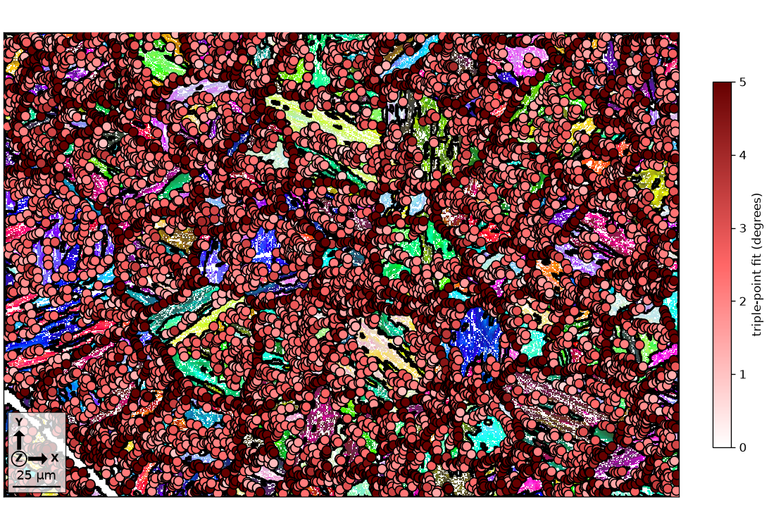
The 20th, 40th, 60th, and 80th triple-point fit percentiles are 2.648, 3.232, 4.015, and 6.295 degrees. Large-fit points often join into parent outlines. Low-fit points support removing all three child boundaries.

Build and cluster the triple-point similarity matrix

Convert the common-parent fit to similarity with a 3-degree threshold and 2-degree tolerance. Every one of the three grain pairs at a triple point receives the same value.

tripleThreshold = 3 * degree
tripleTolerance = 2 * degree

tripleProbability = 1 - 0.5 * (1 + erf(2 * (tripleFit - tripleThreshold) / tripleTolerance))
tripleProbabilityQuantiles = np.nanquantile(tripleProbability, [0.1, 0.5, 0.9])
print(tripleProbabilityQuantiles)

n = len(grains)
g = tP.grainId - 1
tripleA = coo_matrix((tripleProbability, (g[:, 0], g[:, 1])), shape=(n, n)).tocsr()
tripleA = tripleA.maximum(coo_matrix((tripleProbability, (g[:, 1], g[:, 2])), shape=(n, n)).tocsr())
tripleA = tripleA.maximum(coo_matrix((tripleProbability, (g[:, 0], g[:, 2])), shape=(n, n)).tocsr())

tripleInflationPower = 1.4
tripleA = mclComponents(tripleA, tripleInflationPower)

tripleParentGrains = grains.merge(tripleA)
tripleParentId = grains.parentId
tripleParentGrains = smoothBoundary(tripleParentGrains, 20)
numTripleComponents = len(tripleParentGrains)
print(numTripleComponents)

tripleParentEBSD = ebsd.copy()
old2new = np.r_[0, tripleParentId]
tripleParentEBSD.grainId = old2new[ebsd.grainId]

plot(ebsd['Iron bcc'], ebsd['Iron bcc'].orientations, figSize='large')
hold(True)
plot(tripleParentGrains.boundary, lineWidth=2)
hold(False)

[0.     0.6765 0.9651]
657

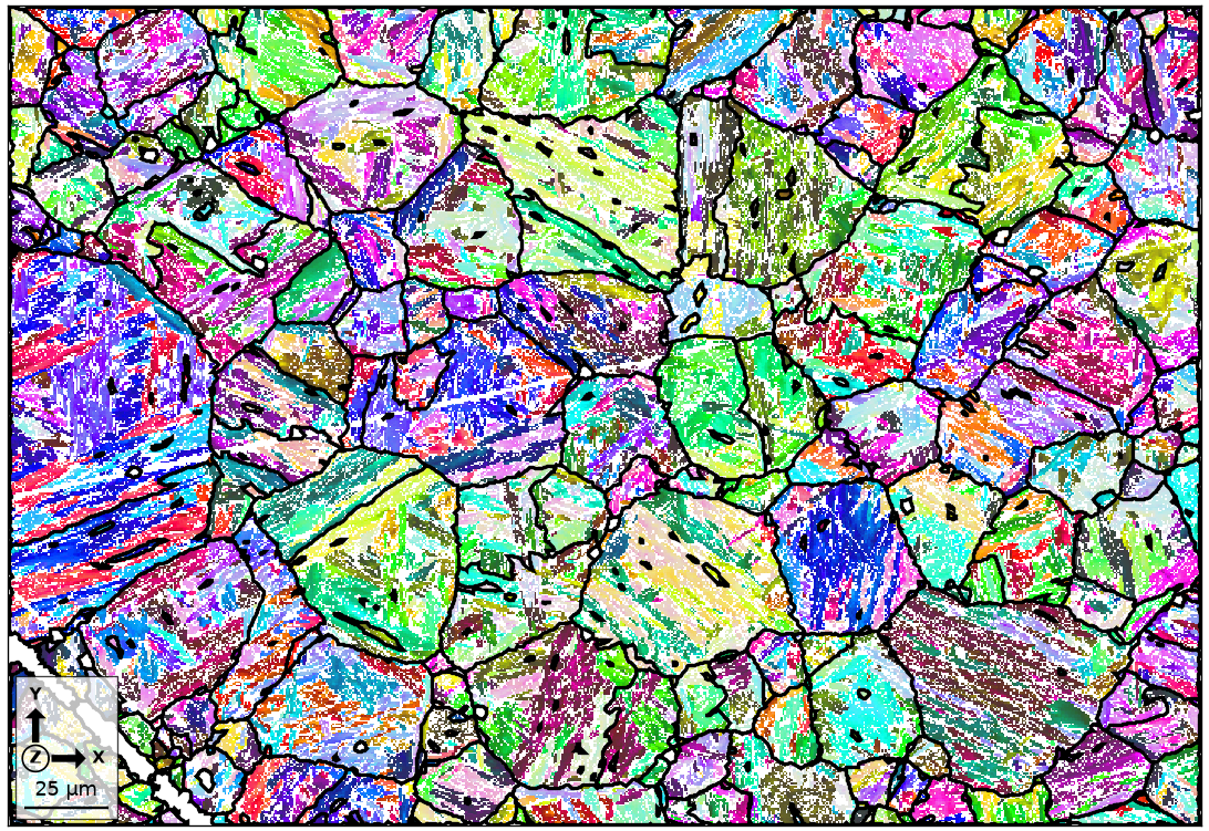
The triple-point probability has 10th, 50th, and 90th percentiles of 0, 0.2032, and 0.8536. Clustering produces 779 candidate parent footprints. Their outlines are shown above. At this stage they still carry child orientations and phases. Fit their common parent orientations, reject weak components, remap the pixels, and merge similar parents with the same sequence used above.

Triple-point graph thresholds

• Common-parent fit pruning inside calcParent: 5 degrees.
• Triple-point similarity: 3-degree threshold and 2-degree tolerance.
• Triple-point graph inflation power: 1.4.

Technical Details

Two things separate the numbers here from the text. The port’s calcParent2Child reaches a lower misfit basin (first quintile 1.22 against 1.48 degrees), and every count after the fit follows the fitted relationship. And the segmentation with removeQuadruplePoints gives 4,467 grains and 11,233 retained pairs where MATLAB has 4,443 and 11,290, a difference of the quadruple point removal rather than of this page, which the Markov clustering amplifies: with MATLAB’s fitted relationship set by hand the page gives 725 boundary components against 707, 361 accepted against 360, and the triple-point fits and similarities to three digits (2.646, 3.227, 4.013 degrees for the first three quintiles).

References

• T. Nyyssönen, P. Peura, and V.-T. Kuokkala, Crystallography, morphology, and martensite transformation of prior austenite in intercritically annealed high-aluminum steel, Metallurgical and Materials Transactions A 49 (2018), 6426-6441, develops the reconstruction and morphology ideas used by this low-level graph workflow.
• T. Nyyssönen, M. Isakov, P. Peura, and V.-T. Kuokkala, Iterative determination of the orientation relationship between austenite and martensite from a large amount of grain pair misorientations, Metallurgical and Materials Transactions A 47 (2016), 2587-2590, gives the OR-fitting method used here.

Next

Continue with Fitting the Orientation Relationship for tools that diagnose, refine, and compare OR models beyond this reconstruction-specific fit.

@article{bachmann2010mtex,
  author  = {F. Bachmann and R. Hielscher and H. Schaeben},
  title   = {Texture Analysis with MTEX - Free and Open Source Software Toolbox},
  journal = {Solid State Phenomena},
  volume  = {160},
  pages   = {63-68},
  year    = {2010},
  doi     = {10.4028/www.scientific.net/SSP.160.63},
  url     = {https://doi.org/10.4028/www.scientific.net/SSP.160.63}
}