
An orientation relationship (OR) is the rotation that relates the parent crystal frame to
the child crystal frame during a phase transition. calcParent2Child
estimates this rotation when only the child phase remains in an EBSD map.
The fit uses misorientations between neighbouring child grains. It assumes that most
retained pairs are variants from a common parent grain. This page first fits and checks an
OR, then explains the objective and the convergence of the algorithm. The full derivation
and implementation decisions are recorded in docs/adr/0005-parent-to-child-fit.md.
import matplotlib.pyplot as plt
import numpy as np

from mtex import *

plottingConvention.default('y↑→x')
Prepare the child-grain pairs
Load the martensite map and segment its bcc measurements into grains. A grain is a phase-homogeneous, spatially connected region of EBSD pixels.
ebsd = mtexdata('martensite', verbose=False)

grains = calcGrains(ebsd, angle=3 * degree, minPixel=2, alpha=12)

job = parentGrainReconstructor(ebsd, grains)
csParent = job.csParent
csChild = job.csChild
neighbors returns pairs of child grains that share a boundary.
The mean orientations of each pair give one child-to-child misorientation.
grainPairs = job.grains[csChild].neighbors()
oriChild = job.grains.selectByGrainId(grainPairs).meanOrientation.reshape(-1, 2)
mori = inv(oriChild[:, 0]) * oriChild[:, 1]
Pairs below 5 degrees are usually subgrain boundaries or the same variant. They cannot constrain the OR and are removed before fitting.
mori = mori[mori.angle() >= 5 * degree]
Fit from all possible starting regions
An ideal Kurdjumov-Sachs (KS) relationship is a useful initial candidate. By default,
calcParent2Child also scans the complete fundamental region. It refines the best
candidates and returns the one with the lowest misfit.
p2cKS = orientation.KurdjumovSachs(csParent, csChild)
print(p2cKS)
p2cGlobal, fitGlobal = calcParent2Child(mori, p2cKS, fit=True)
p2cGlobal
misorientation (Iron fcc → Iron bcc (old))
  (111) || (011)   [101̅] || [111̅]
 optimizing parent to child orientation relationship
  scanning 398 orientations
  (102.23°,  8.99°,303.54°)  2.291
  (102.35°,  8.96°,303.47°)  2.287
  (102.36°,  8.96°,303.47°)  2.287
misorientation (Iron fcc → Iron bcc (old))
  Bunge Euler angles in degree
  phi1   Phi  phi2
   347  8.97  56.8
Inspect the residuals
The second output contains one residual for every input misorientation. A residual is the disorientation to the closest predicted child-to-child variant, excluding the identity variant.
plt.close('all')
plt.hist(fitGlobal / degree, bins=50)
plt.axvline(np.nanquantile(fitGlobal, 0.9) / degree, color='k', linestyle='--', label='90% cutoff')
plt.legend()
plt.xlabel('disorientation to the closest variant in degrees')
plt.ylabel('number of neighbouring grain pairs')
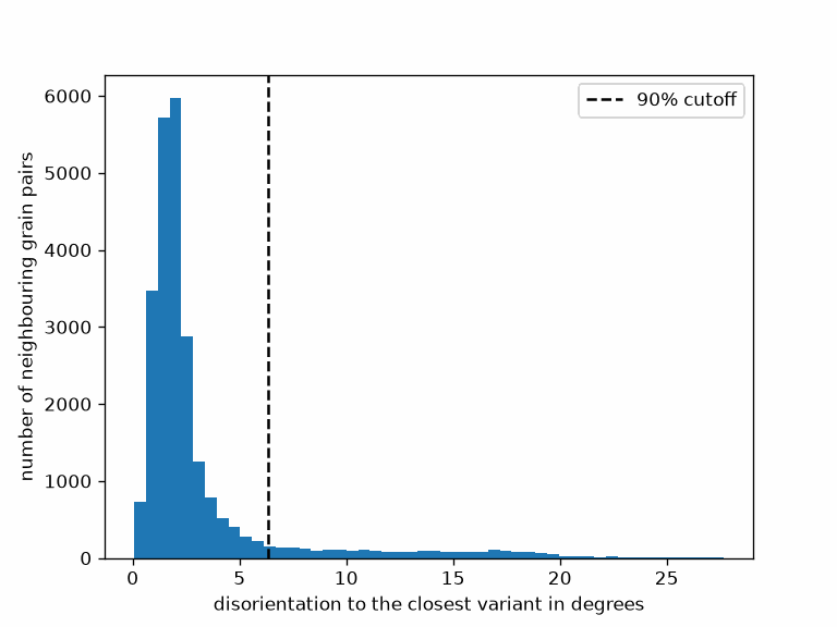
Notice the main population at small residuals and the longer tail. Not every neighbouring pair belongs to one former parent grain. The default fit therefore uses the best 90 percent rather than allowing the tail to pull an ordinary mean away from the main population.
The quantile option changes that retained fraction. The threshold option caps the loss
of larger residuals. Use a threshold in degrees only when the experiment supplies a
defensible angular tolerance; otherwise the default quantile needs no new scale.
Compare local and global fits
The local option skips the scan and starts the fixed-point iteration at the supplied
relationship. It is useful when the starting OR is already trusted.
p2cLocal = calcParent2Child(mori, p2cKS, local=True)
print(p2cLocal)
localToGlobal = angle(p2cLocal, p2cGlobal) / degree
localToGlobal
 optimizing parent to child orientation relationship
  (335.80°, 10.53°, 65.80°)  4.011
  (339.00°, 10.45°, 63.23°)  3.568
  (341.88°, 10.74°, 61.13°)  3.087
  (344.84°, 10.65°, 58.59°)  2.806
  (346.44°, 10.46°, 57.26°)  2.693
  (347.25°, 10.34°, 56.61°)  2.658
  (347.58°, 10.28°, 56.35°)  2.65
  (347.71°, 10.26°, 56.25°)  2.648
  (347.00°, 10.01°, 57.10°)  2.604
  (347.14°,  9.91°, 57.08°)  2.558
  (346.71°,  9.31°, 57.61°)  2.348
  (347.39°,  8.97°, 56.82°)  2.284
misorientation (Iron fcc → Iron bcc (old))
  Bunge Euler angles in degree
  phi1   Phi  phi2
   347  8.97  56.8
0
The printed value is the angular separation of the two fitted ORs. The global solution is a good degree away from the KS-started local result and gives the lower objective value. That difference is not negligible when habit planes are computed from the fitted relationship.
Nishiyama-Wassermann, Pitsch, and Greninger-Trojano starting relationships all reach the better basin on this map; Kurdjumov-Sachs does not. The complete scan is therefore the default. The supplied starting OR remains one candidate, so scanning cannot discard a better local result. It costs about two and a half times one local fit on this data.
The scan is deterministic. Its subsamples stride through an angle-sorted list instead of
drawing at random, so repeated fits to the same data return the same result. A local fit
reaches a stationary point rather than a guaranteed best fit, so its starting relationship
can decide the answer. Use local when refining a trusted OR or fitting many small data
sets in a loop, where the fixed cost of the scan dominates.
The model: child variants determine the observed misorientations
A variant is one crystallographically equivalent child
orientation predicted from a single parent orientation by a known OR. For a parent
orientation oriParent, the possible child variants have the form p2c * S, where S
runs through the parent point group.
Two child grains from one parent may select different variants. Their possible child-to-child misorientations are the following set.
p2cVariants = p2cGlobal.variants().reshape(-1)
c2c = p2cGlobal * inv(p2cVariants)
c2c
misorientation (Iron bcc (old) → Iron bcc (old))
  size: 24
  Bunge Euler angles in degree
  phi1   Phi   phi2
     0     0      0
   318   105    222
   221    77   38.9
  89.1   176   90.9
   141    77    319
     ⋮     ⋮      ⋮
   322  93.2    312
   179   162  0.649
  38.7  88.1   53.2
   139  89.6    230
   347  17.9    193
In symbols, each member is p2c * inv(S) * inv(p2c). This is the parent point group
conjugated by p2c. Conjugation leaves the rotation angles unchanged. Without child
symmetry reduction, a cubic parent supplies only 0, 90, 120, and 180 degree rotations.
np.unique(np.round(angle(c2c, symmetry=False) / degree))
array([ 0., 90., 120., 180.])
Only the rotation axes depend on the OR. Child symmetry reduces each misorientation to its disorientation, which spreads those four angles into the longer list below. The list belongs to the fitted relationship, not to ideal KS, whose disorientation angles are 10.53, 14.88, 20.61, 21.06, 47.11, 49.47, 50.51, 51.73, 57.21, and 60 degrees.
np.unique(np.round(angle(c2c) / degree, 2))
array([ 0.  ,  4.11,  9.84, 12.68, 15.17, 17.61, 17.95, 50.9 , 51.29,
       51.84, 52.51, 52.9 , 56.12, 56.26, 56.77, 59.82, 60.34])
See the axis fit
The coloured density shows axes of the measured child-to-child misorientations. Black squares mark axes predicted by the fitted OR.
plot(mori.axis(), contourf=True, fundamentalRegion=True, halfwidth=5 * degree)
hold(True)
isInformative = angle(c2c) > 1e-3 * degree
plot(c2c[isInformative].axis(), marker='s', markerFaceColor='none', markerEdgeColor='k', markerSize=8)
hold(False)
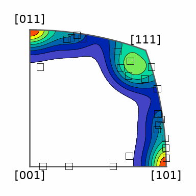
Notice that the black squares lie on the main measured axis clusters. Fitting an OR is therefore mainly an axis-alignment problem: it rotates the parent’s symmetry axes onto those observed clusters.
The predicted set also contains the identity rotation at zero degrees. It is produced by
S = identity for every possible OR and carries no information about the fit.
calcParent2Child excludes this identity variant.
The objective function
For a candidate OR, the residual of each observation is its disorientation to the closest informative child-to-child variant.
omega = np.min(angle(mori.reshape(-1, 1), c2c[isInformative].reshape(1, -1)), axis=1)
calcParent2Child minimises a trimmed chordal misfit. It averages 1 - cos(omega) over the
best quantile fraction of the observations, which is 90 percent by default. This robust
objective limits the influence of pairs from different parents.
The misfit is unchanged when p2c is multiplied by child symmetry on the left or parent
symmetry on the right. Its search domain is therefore the misorientation fundamental region
of the phase pair. For cubic-to-cubic symmetry its volume is 8*pi^2/(24*24), or about
0.137 radians cubed. The domain is only three-dimensional, which makes a complete scan
practical.
The fixed-point algorithm
Each observation becomes a direct measurement of the OR once a variant has been assigned.
If mori exactly equals the variant c2c(k), the following product returns p2cGlobal
itself.
k = 5
c2c[k - 1] * p2cVariants[k - 1]
misorientation (Iron fcc → Iron bcc (old))
  Bunge Euler angles in degree
  phi1   Phi  phi2
   347  8.97  56.8
A noisy observation therefore votes for an OR near the true one. Averaging many such votes averages away part of the noise. One iteration performs four operations:
- assign every misorientation to its closest variant;
- keep the best
quantilefraction; - form the vote
mori * p2cVariants(k)for each retained pair; and - replace
p2cby the mean of the votes.
The vote depends on the current p2c, so this is a fixed-point iteration rather than a
descent step. The misfit need not decrease at every step. The implementation therefore
backtracks whenever a full step does not lower the objective.
Why the iteration converges
Write p2c = pStar * exp(xi) for a small error xi around the solution. A vote from
variant k has error R_k' * xi, where R_k is the matrix of the corresponding parent
symmetry operation. One iteration maps the error with
where w_k is the fraction assigned to variant k. The matrix A is an average of
rotation matrices, so its norm cannot exceed one and the local iteration cannot diverge.
For evenly populated variants, the parent-group matrices sum to zero.
R = csParent.properGroup().rot
Aeven = np.sum(R.matrix().reshape(-1, 3, 3), axis=0)
np.linalg.norm(Aeven, 2)
3.4736e-15
This cancellation follows from group theory. The three-dimensional vector representation of the cubic rotation group has no copy of the trivial representation. A martensitic microstructure usually populates many variants, so the error contracts in only a handful of iterations.
Removing the identity operation gives A = -I/23 for even occupancy. Its convergence rate
is therefore 1/23 per iteration. On this map the variant occupancies range from 1.5 to 12
percent, and the measured local rate is about 0.24 per iteration.
The iteration stalls only if A has an eigenvalue with modulus one. That requires every
populated variant to share a common rotation axis. Two populated variants with non-parallel
axes are enough to rule this out.
What the classical damping factor does
Classical implementations average the old and new estimates, using a weight alpha on the
old estimate. In the linearised error map this replaces A by
An eigenvalue lambda becomes (alpha + lambda)/(1 + alpha). The damping factor can
therefore cancel a negative real eigenvalue exactly. This explains the traditional
alpha = 1/numSym(csParent) default. For even occupancy the eigenvalue is -1/23, and
1/24 nearly cancels it.
Its benefit depends on the spectrum of A:
| occupancy | rho(0) | best alpha | rho(alpha) |
|---|---|---|---|
| even over all 23 variants | 0.0435 | 0.043 | 0.0000 |
| only the 180 degree variants | 0.3333 | 0.334 | 0.0001 |
| only the 120 degree variants | 0.0000 | 0.000 | 0.0000 |
| only the 90 degree variants | 0.3333 | 0.000 | 0.3333 |
The last row is the important counterexample. Fourfold operations give A complex
eigenvalues, and a real shift cannot move that conjugate pair towards zero. Damping treats
oscillation along a direction, not rotation between directions.
On this map the eigenvalues are -0.238, -0.099, and 0.021. Theory predicts that
alpha = 0.11 would roughly halve the asymptotic rate. Measured from several starting
points, however, no tested damping shortened the fit. Undamped fits needed 12, 23, and 18
iterations. With alpha = 1/24 they needed 13, 24, and 19 iterations. With alpha = 1/4
they needed 15, 22, and at least 25 iterations. The middle alpha = 1/4 fit had not
converged at the iteration cap. All runs stopped at the same misfit.
The asymptotic rate governs only the final digits. Early iterations are dominated by changing variant assignments and changing membership of the trimmed set. Damping merely shortens those early steps. MTEX therefore leaves the iteration undamped and uses backtracking for steps that do not descend.
Technical Details
The port’s fit is the same objective with its own iteration, and on this map it does better than the text above says: the local fit from Kurdjumov-Sachs already reaches the lower basin, so the local and the global result agree to a few hundredths of a degree, and both have the trimmed misfit 7.948e-4 where MATLAB’s global fit has 7.957e-4 and its KS-started local fit 1.068e-3; the two global results lie 0.22 degrees apart. The scan scores its candidates on a subsample, so the start refined on all the data is compared with the winner at the end.
References
- T. Nyyssönen, M. Isakov, P. Peura, and V.-T. Kuokkala, Iterative determination of the orientation relationship between austenite and martensite from a large amount of grain pair misorientations, Metallurgical and Materials Transactions A 47 (2016), 2587-2590, gives the iterative OR-fitting method.
- T. Nyyssönen, P. Peura, and V.-T. Kuokkala, Crystallography, morphology, and martensite transformation of prior austenite in intercritically annealed high-aluminum steel, Metallurgical and Materials Transactions A 49 (2018), 6426-6441, provides the reconstruction setting used by the example.
Citing this page.
This page is part of the documentation of
MTEX, a free and open
source MATLAB toolbox for analyzing and modeling crystallographic textures.
It was written by The MTEX Developers and is published at
https://mtex-toolbox.github.io/OrientationRelationshipFit_py.html.
If you use MTEX, or reuse text or figures from this page, in your research,
please cite
F. Bachmann, R. Hielscher, H. Schaeben: Texture Analysis with MTEX - Free and Open Source Software Toolbox, Solid State Phenomena 160 (2010), 63-68. 10.4028/www.scientific.net/SSP.160.63
BibTeX
@article{bachmann2010mtex,
  author  = {F. Bachmann and R. Hielscher and H. Schaeben},
  title   = {Texture Analysis with MTEX - Free and Open Source Software Toolbox},
  journal = {Solid State Phenomena},
  volume  = {160},
  pages   = {63-68},
  year    = {2010},
  doi     = {10.4028/www.scientific.net/SSP.160.63},
  url     = {https://doi.org/10.4028/www.scientific.net/SSP.160.63}
}
Other papers describing specific MTEX methods are listed under Publications — please cite the one that best fits your application. The MTEX source code is licensed under the GNU General Public License v2.0; the text and figures of this documentation are licensed under CC BY 4.0, which permits reuse — including by automated systems — provided The MTEX Developers and this page are credited.