Parent and Child Variants

The stable crystallographic structure of most materials depends on conditions such as temperature and pressure. A solid-state phase transition changes that structure when the conditions change.

The initial lattice is the parent phase, and the resulting lattice is the child phase.

The two phases can have the same chemical composition but different crystal structures. In titanium, the parent beta phase is cubic and the child alpha phase is hexagonal.

import numpy as np

from mtex import *

plottingConvention.default('y↑→x')

csBeta = crystalFrame('432', [3.3, 3.3, 3.3], mineral='Ti (beta)')
csAlpha = crystalFrame('622', [3, 3, 4.7], mineral='Ti (alpha)')

The Burgers orientation relationship

An orientation relationship (OR) is a fixed angular relation between the parent and child lattices. Atomic rearrangement during the transition makes some plane and direction alignments energetically favourable.

Let oriParent describe the lattice before the transition.

oriParent = orientation.rand(csBeta)

The dominant OR between beta and alpha titanium is the Burgers OR. MTEX stores it as a parent-to-child orientation.

beta2alpha = orientation.Burgers(csBeta, csAlpha)
beta2alpha

misorientation (Ti (beta) → Ti (alpha))
  (110) || (0001)   [1̅11̅] || [21̅1̅0]

A child orientation consistent with this OR is obtained by multiplying the parent orientation by the inverse OR.

oriChild = oriParent * inv(beta2alpha)
oriChild

orientation (Ti (alpha) → y↑→x)
  Bunge Euler angles in degree
  phi1   Phi  phi2
   287  17.3   324

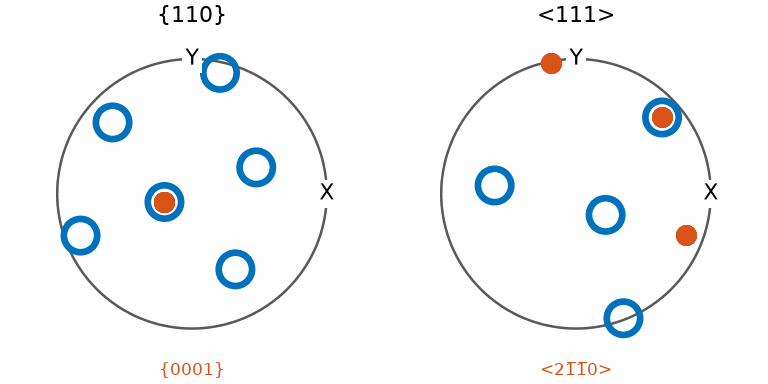
The Burgers OR aligns a hexagonal \((0001)\) plane with a cubic \((110)\) plane. It also aligns a hexagonal \([2\bar{1}\bar{1}0]\) direction with a cubic \([\bar{1}1\bar{1}]\) direction.

The two pole figures below check those parallelisms for oriParent and oriChild.

In the left panel all twelve small child poles fall on a large parent pole. The plane alignment survives every symmetric copy. The right panel is different: only four of the twelve child directions land on a parent pole, and the rest sit 10.5 or 49.5 degrees away. The six equivalent basal directions are 60 degrees apart, while the two cubic axes lying in the same plane are 70.5 degrees apart, so a direction alignment cannot repeat for every copy the way a plane alignment does.

# (110) / (0001) pole figure
plotPF(oriParent, Miller(1, 1, 0, csBeta), markerSize=20, markerFaceColor='none', lineWidth=4, layout=[1, 2])
hold(True)
plot(oriChild.symmetrise() * Miller(0, 0, 0, 1, csAlpha), markerSize=12)
xlabel(Miller(0, 0, 0, 1, csAlpha).char(), color=ind2color(1))
hold(False)

# [111] / [2-1-10] pole figure
nextAxis(1)
plotPF(oriParent, Miller(1, 1, 1, csBeta, 'uvw'), upper=True, markerSize=20, markerFaceColor='none', lineWidth=4)

dAlpha = Miller(2, -1, -1, 0, csAlpha, 'uvw')
hold(True)
plot(oriChild.symmetrise() * dAlpha, markerSize=12)
xlabel(dAlpha.char(), color=ind2color(1))
hold(False)
gcm().drawNow()

Define an OR from parallel features

The same alignment rules can define the OR directly with orientation.map.

beta2alpha = orientation.map(Miller(1, 1, 0, csBeta), Miller(0, 0, 0, 1, csAlpha),
                             Miller(-1, 1, -1, csBeta, 'uvw'), Miller(2, -1, -1, 0, csAlpha, 'uvw'))

Defining the OR through crystal planes and directions has an important advantage. The definition does not depend on the hexagonal crystal-frame convention.

Child variants

A variant is one crystallographically equivalent child orientation predicted from a single parent orientation by a known OR. It is the finest-grained classification of a child relative to its parent.

Cubic proper symmetry gives oriParent 24 equivalent representations.

oriParentSym = oriParent.symmetrise()
oriParentSym.size

24

Applying the OR to all 24 representations gives 24 child orientations.

oriChild = oriParentSym * inv(beta2alpha)
oriChild.size

24

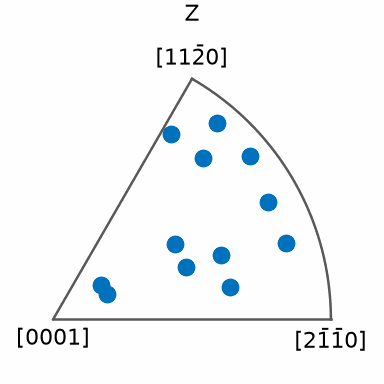
Under hexagonal child symmetry, some of these orientations represent the same physical orientation. For the exact Burgers OR they form 12 pairs.

The inverse pole figure places both members of each pair at the same location. The 24 computations therefore appear as only 12 distinct points.

plotIPF(oriChild, vector3d.Z)

variants removes the symmetry-equivalent duplicates directly. It returns the 12 child variants for this OR.

oriChild = variants(beta2alpha, oriParent)

for i in range(1, 13):
  plotIPF(oriChild[i - 1], ind2color(i - 1), vector3d.Z, label=i, markerEdgeColor='k')
  hold(True)
hold(False)

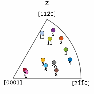
The labels are variant IDs. A variant ID is an index into this ordered set, so specific variants can be selected by passing their IDs.

oriChild = variants(beta2alpha, oriParent, [2, 3])
oriChild

orientation (Ti (alpha) → y↑→x)
  size: 2
  Bunge Euler angles in degree
  phi1   Phi  phi2
   347  98.8  99.7
   112  42.7   208

Exact and approximate orientation relationships

The reduction from 24 parent representations to 12 variants is specific to the exact Burgers OR. A general OR between these two phases has exactly 24 variants.

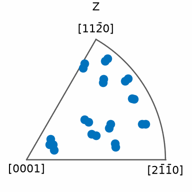
Disturbing the Burgers OR by a fixed 2 degree rotation breaks the exact pairing.

beta2alpha = beta2alpha * orientation.byAxisAngle(vector3d(1, 2, 3), 2 * degree, csBeta, csBeta)

The inverse pole figure now contains 24 points. They remain close to the 12 exact Burgers positions, so each former pair appears slightly split. variants treats two representations as the same when they agree to within about 1.6 degrees, which is why the perturbation has to exceed that for the pairs to separate.

oriChildPerturbed = variants(beta2alpha, oriParent)
print(oriChildPerturbed.size)
plotIPF(oriChildPerturbed, vector3d.Z)

24

Identify an observed variant

The inverse task is to determine a variant ID from a parent-child pair or from two child orientations. The calcVariants method does this after a parent grain reconstruction has been computed.

That workflow is demonstrated in Parent Austenite Reconstruction.

Parent variants

The same ambiguity occurs in the opposite direction. Given one child orientation, several parent orientations could have produced it. variants returns them with 'parent'.

# return to the exact Burgers orientation relationship
b2a = orientation.Burgers(csBeta, csAlpha)

# select one child variant
oriChildSingle = variants(b2a, oriParent, 1)

oriParents = variants(b2a, oriChildSingle, 'parent')
oriParents.size

6

There are six parent variants, compared with 12 child variants. The two counts need not agree because the parent and child point-group orders govern them differently.

One of the six is the parent orientation from which the child was made. The minimum misorientation below is therefore zero degrees to numerical precision.

np.min(angle(oriParents, oriParent)) / degree

2.4841e-14

The parents method returns the same set of OR variants. Multiplying the child orientation by them produces the six candidate parent orientations.

unique(oriChildSingle * b2a.parents())

orientation (Ti (beta) → y↑→x)
  size: 6
  Bunge Euler angles in degree
  phi1   Phi  phi2
   184  38.5   156
  24.5  73.3   122
  47.6  26.4   285
  64.5    18  89.6
    22  83.5   302
   189  48.4   332

A single child orientation cannot identify which candidate parent is correct. Parent grain reconstruction resolves the ambiguity by comparing neighbouring child grains.

References

• W. G. Burgers, On the process of transition of the cubic-body-centered modification into the hexagonal-close-packed modification of zirconium, Physica 1 (1934), 561-586, establishes the plane and direction relations used here.

Next

Continue with Martensite Variants to classify variants, packets, and Bain groups in a measured steel microstructure.

@article{bachmann2010mtex,
  author  = {F. Bachmann and R. Hielscher and H. Schaeben},
  title   = {Texture Analysis with MTEX - Free and Open Source Software Toolbox},
  journal = {Solid State Phenomena},
  volume  = {160},
  pages   = {63-68},
  year    = {2010},
  doi     = {10.4028/www.scientific.net/SSP.160.63},
  url     = {https://doi.org/10.4028/www.scientific.net/SSP.160.63}
}