
This page assumes the directions introduced in Defining Three-Dimensional Vectors and the active rotations introduced in Defining Rotations.
A reference frame is the coordinate system in which data are expressed. The rotations below move objects within one reference frame. They do not perform a frame change, which re-expresses the same physical object in a different reference frame without moving it.
The examples use proper rotations. Reflections and inversions are covered in Improper Rotations.
import numpy as np
from mtex import *
plottingConvention.default('y↑→x')
Rotating a Direction
The product rot * v actively turns the direction v by rot.
rot = rotation.byEuler(90 * degree, 90 * degree, 0 * degree, 'Bunge')
v = rot * vector3d.X
v
vector3d (y↑→x)
  x  y  z
  0  1  0
The grey arrows are the specimen axes. The black arrow is X before the rotation, and the red arrow is its image.
arrow3d(1.2 * cat(vector3d.X, vector3d.Y, vector3d.Z), faceColor=[.75, .75, .75])
hold(True)
arrow3d(1.05 * vector3d.X, faceColor='black')
arrow3d(1.05 * v, faceColor='red')
hold(False)
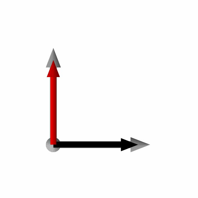
The red arrow coincides with Y, so this rotation sends X to Y. The inverse rotation,
inv(rot) * v (MATLAB’s rot \ v), returns the direction to X.
inv(rot) * v
vector3d (y↑→x)
  x  y  z
  1  0  0
Composing Rotations
Multiplication composes rotations. The rotation on the right acts first, just as it does in matrix multiplication.
rot1 = rotation.byEuler(90 * degree, 0, 0, 'Bunge')
rot2 = rotation.byEuler(0, 60 * degree, 0, 'Bunge')
rot = rot2 * rot1
The order matters. == tests rotation equality within an angular tolerance, rather than comparing printed Euler angles. Reversing these two rotations does not give the same result.
rot2 * rot1 == rot1 * rot2
False
Their angular separation is 82.8192 degrees.
angle(rot2 * rot1, rot1 * rot2) / degree
82.8192
The black arrow below is one starting direction. The red arrow results from rot1
followed by rot2, while the blue arrow shows the reverse order.
startDirection = normalize(vector3d(1, 1, 1))
forwardDirection = rot2 * (rot1 * startDirection)
reverseDirection = rot1 * (rot2 * startDirection)
arrow3d(1.2 * cat(vector3d.X, vector3d.Y, vector3d.Z), faceColor=[.75, .75, .75])
hold(True)
arrow3d(1.05 * startDirection, faceColor='black')
arrow3d(1.05 * forwardDirection, faceColor='red')
arrow3d(1.05 * reverseDirection, faceColor='blue')
hold(False)
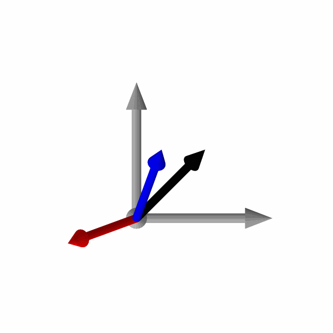
The separated red and blue arrows make the noncommutativity visible. Parentheses are useful whenever the intended order might otherwise be misread.
Axis and Angle
angle and axis read the axis–angle description from the composed rotation, however it was built.
rot.angle() / degree
104.4775
rot.axis()
vector3d (y↑→x)
      x       y      z
  0.447  -0.447  0.775
The composite is a 104.4775 degree turn about the displayed axis. This is not the sum of the two input angles because rotations about different axes do not add like vectors.
The Inverse Rotation
inv reverses a rotation. For a nonzero turn below 180 degrees, the inverse has the opposite axis and the same canonical, nonnegative angle.
invRot = inv(rot)
cat(rot.axis(), invRot.axis())
vector3d (y↑→x)
  size: 2
       x       y       z
   0.447  -0.447   0.775
  -0.447   0.447  -0.775
np.array([rot.angle(), invRot.angle()]) / degree
array([104.4775, 104.4775])
A rotation multiplied by its inverse is the identity. This is why inv(rot) * v undoes
rot * v.
rot * invRot
rotation
  Bunge Euler angles in degree
  phi1  Phi  phi2
     0    0     0
The Angle Between Two Rotations
The relative rotation below acts after rot1 and carries its result to the result of
rot. Its principal angle is the angular distance between the two rotations.
relativeRot = rot * inv(rot1)
np.array([relativeRot.angle(), angle(rot, rot1)]) / degree
array([60., 60.])
Both entries are 60 degrees. The second is the direct angle(rot,rot1) call, so there is usually no need to construct the relative rotation explicitly.
This angular distance is used throughout MTEX to compare a fit with a measurement and to quantify orientation variation. For orientations it additionally minimizes over symmetry-equivalent descriptions, as explained in Orientation Symmetry.
Lists of Rotations
MTEX objects are vectorized. If both operands are non-scalar, * pairs corresponding
entries by NumPy broadcasting; a column of rotations times a row of directions forms
every combination. A scalar operand is applied to the whole list.
rotations = rotation.byAxisAngle(vector3d.Z, np.array([0, 30, 60]) * degree)
directions = cat(vector3d.X, vector3d.Y, vector3d.Z)
(rotations * directions).shape
(3,)
The elementwise result has three entries: one output for each pair.
(rotations.reshape(-1, 1) * directions).shape
(3, 3)
The outer result has size 3-by-3: every rotation was applied to every direction. The same distinction applies when two rotation lists are composed.
Reading Other Parametrisations
A rotation can be inspected in any representation, regardless of how it was constructed.
| Euler(rot) | the three Euler angles |
| Rodrigues(rot) | the Rodrigues–Frank vector |
| matrix(rot) | the rotation matrix |
| homochoric(rot) | the homochoric vector |
| cubochoric(rot) | the cubochoric vector |
| axis(rot), angle(rot) | axis and angle |
Euler angles depend on a convention. Naming Matthies here makes the result independent of the user’s display preference.
alpha, beta, gamma = Euler(rot, 'Matthies')
np.array([alpha, beta, gamma]) / degree
array([270., 60., 180.])
The displayed 270, 60, 180 degree triplet is the Matthies description of the same composite rotation. See Rotation Representations before comparing coordinates produced by different programs.
The Maths Behind the Angular Distance
For rotations \(r_1\) and \(r_2\), MTEX uses the principal angle of a relative rotation:
\[d(r_1,r_2) = \mathop{\rm angle}(r_2 r_1^{-1}) = \mathop{\rm angle}(r_1^{-1}r_2).\]The two relative rotations generally have different axes, but they have the same angle.
The distance is unchanged if the same rotation is composed onto both inputs from the
left or from the right. This invariance is why the 60 degree result above does not
depend on the starting orientation rot1.
References
- A. Morawiec, Orientations and Rotations: Computations in Crystallographic Textures, Springer, 2004, develops composition and the geometry of rotation space for texture analysis.
- D. Rowenhorst et al., Consistent representations of and conversions between 3D rotations, Modelling and Simulation in Materials Science and Engineering 23 (2015) 083501, documents the convention choices behind common parametrisations.
Next
Sets of rotations are drawn in Plotting. A rotation that maps crystal coordinates into specimen coordinates and carries crystal symmetry is an orientation.
Technical Details
Python has no \ operator, so the inverse rotation is applied as inv(rot) * v. The
product of two lists follows NumPy broadcasting: MATLAB’s .* is * on lists of one
shape, MATLAB’s outer * is a column times a row.
Citing this page.
This page is part of the documentation of
MTEX, a free and open
source MATLAB toolbox for analyzing and modeling crystallographic textures.
It was written by The MTEX Developers and is published at
https://mtex-toolbox.github.io/RotationOperations_py.html.
If you use MTEX, or reuse text or figures from this page, in your research,
please cite
F. Bachmann, R. Hielscher, H. Schaeben: Texture Analysis with MTEX - Free and Open Source Software Toolbox, Solid State Phenomena 160 (2010), 63-68. 10.4028/www.scientific.net/SSP.160.63
BibTeX
@article{bachmann2010mtex,
  author  = {F. Bachmann and R. Hielscher and H. Schaeben},
  title   = {Texture Analysis with MTEX - Free and Open Source Software Toolbox},
  journal = {Solid State Phenomena},
  volume  = {160},
  pages   = {63-68},
  year    = {2010},
  doi     = {10.4028/www.scientific.net/SSP.160.63},
  url     = {https://doi.org/10.4028/www.scientific.net/SSP.160.63}
}
Other papers describing specific MTEX methods are listed under Publications — please cite the one that best fits your application. The MTEX source code is licensed under the GNU General Public License v2.0; the text and figures of this documentation are licensed under CC BY 4.0, which permits reuse — including by automated systems — provided The MTEX Developers and this page are credited.