
The same rotation can be described by different coordinates. The best choice depends on whether the coordinates will be plotted, sampled, or used to build a grid.
This page assumes the axis–angle and quaternion descriptions introduced in Defining Rotations. MTEX stores the proper part of every rotation as a unit quaternion. The coordinates below are computed from that quaternion on demand.
Rodrigues and homochoric coordinates are scaled-axis representations. Their direction is the rotation axis \(\vec n\). Their length is a function \(f(\omega)\) of the principal rotation angle \(0 \leq \omega \leq \pi\):
\[\vec v = f(\omega)\,\vec n.\]Cubochoric coordinates take one further step and map the homochoric ball onto a cube. They therefore do not, in general, point along the rotation axis.
import matplotlib.pyplot as plt
import numpy as np
from mtex import *
rot = rotation.rand(100000)
Rodrigues–Frank Coordinates
The Rodrigues–Frank vector scales the axis by \(f(\omega)=\tan(\omega/2)\). MTEX computes it with Rodrigues.
The following output puts the angle in degrees in the first column and the length of its Rodrigues vector in the second.
sampleAngle = np.array([0, 60, 120, 170, 179]) * degree
sampleRot = rotation.byAxisAngle(vector3d.Z, sampleAngle)
vRodrigues = sampleRot.Rodrigues()
rodriguesLength = norm(vRodrigues)
np.column_stack([sampleAngle / degree, rodriguesLength])
array([[  0.    ,   0.    ],
       [ 60.    ,   0.5774],
       [120.    ,   1.7321],
       [170.    ,  11.4301],
       [179.    , 114.5887]])
The length grows rapidly near a half turn. At exactly \(180^\circ\) it is infinite, so the full rotation space is unbounded in Rodrigues coordinates. Rotations about one fixed axis nevertheless form a straight line, and symmetry boundaries become planes. These properties make Rodrigues coordinates useful for visualizing fundamental regions.
rotation.byRodrigues performs the inverse conversion. The displayed angular error confirms the round trip.
rotFromRodrigues = rotation.byRodrigues(vRodrigues)
np.max(angle(sampleRot, rotFromRodrigues)) / degree
0
Homochoric Coordinates
Rodrigues coordinates simplify geometry but distort volume. Homochoric coordinates instead scale the rotation axis by
\[f(\omega) = \left(\frac{3}{4}\left(\omega-\sin\omega\right)\right)^{1/3}.\]homochoric maps all rotations into a ball. Its radius is \(R=(3\pi/4)^{1/3}\), reached by the half turns.
vHomochoric = rot.homochoric()
R = (0.75 * np.pi) ** (1 / 3)
halfTurn = rotation.byAxisAngle(vector3d.Z, np.pi)
np.array([norm(halfTurn.homochoric()), R])
array([1.3307, 1.3307])
A volume check
rotation.rand samples the uniform, or Haar, distribution on the rotation group. Equal-volume homochoric coordinates turn that sample into a uniform distribution in the ball.
A uniform ball does not have a uniform distribution of radii. A shell at radius \(r\) has more volume than a shell of the same thickness near the centre, so the radial density is \(3r^2/R^3\).
plt.figure()
plt.hist(norm(vHomochoric), 50, density=True)
r = np.linspace(0, R, 100)
plt.plot(r, 3 * r ** 2 / R ** 3, linewidth=2)
plt.legend(['sampled radii', 'uniform-ball density'], loc='upper left')
plt.xlabel('homochoric radius')
plt.ylabel('probability density')
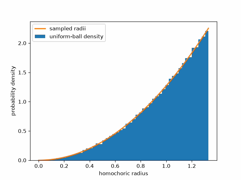
Reading the volume check
The sampled bars follow the increasing theoretical curve. This agreement is the visible consequence of preserving Haar volume. It does not mean that homochoric coordinates preserve angles, shapes, or distances between arbitrary rotations.
Cubochoric Coordinates
Cubochoric coordinates compose the homochoric map with an equal-volume map from the ball to a cube. The cube has edge length \(\pi^{2/3}\) and the same volume, \(\pi^2\), as the homochoric ball.
MTEX computes these coordinates with cubochoric. The next figure maps the same half turns first to the homochoric boundary and then to the cubochoric boundary.
halfTurnAxis = equispacedS2Grid(points=2000)
boundaryRot = rotation.byAxisAngle(halfTurnAxis, np.pi)
homochoricBoundary = boundaryRot.homochoric()
cubochoricBoundary = boundaryRot.cubochoric()
fig = plt.figure(figsize=(9, 4.5))

ax = fig.add_subplot(1, 2, 1, projection='3d')
ax.scatter(homochoricBoundary.x, homochoricBoundary.y, homochoricBoundary.z, s=4)
ax.set_box_aspect((1, 1, 1))
ax.set_xlabel('$h_1$'); ax.set_ylabel('$h_2$'); ax.set_zlabel('$h_3$')
ax.set_title('homochoric boundary')

ax = fig.add_subplot(1, 2, 2, projection='3d')
ax.scatter(cubochoricBoundary.x, cubochoricBoundary.y, cubochoricBoundary.z, s=4)
ax.set_box_aspect((1, 1, 1))
ax.set_xlabel('$c_1$'); ax.set_ylabel('$c_2$'); ax.set_zlabel('$c_3$')
ax.set_title('cubochoric boundary')
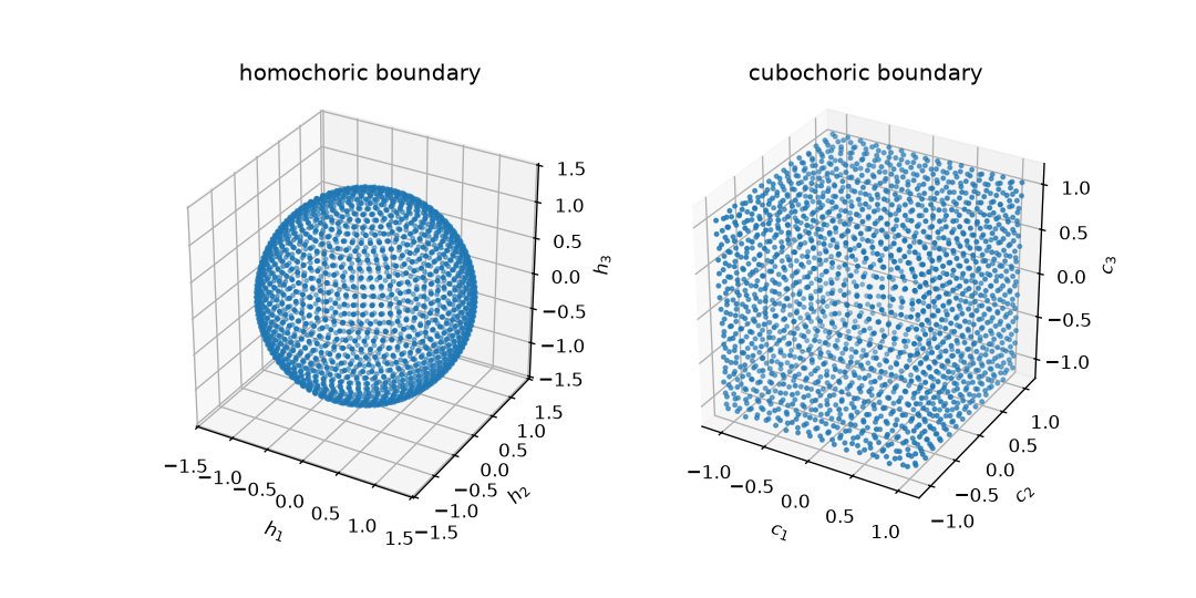
Reading the coordinate domains
The spherical boundary on the left becomes the six faces of the cube on the right. Opposite axes describe the same \(180^\circ\) rotation, so opposite boundary locations are identified. Neither domain is an ordinary solid with independent points everywhere on its boundary.
The cube is convenient for Cartesian grids. This is why homochoricSO3Grid constructs its internal grid in cubochoric coordinates despite the class name.
Inverting Cubochoric Coordinates
MATLAB has no rotation.byCubochoric constructor: it first maps the cube back to the
homochoric ball with cubo2homo, then uses
rotation.byHomochoric. The same route works here.
vCubochoric = rot.cubochoric()
xyz = cubo2homo(np.column_stack([vCubochoric.x, vCubochoric.y, vCubochoric.z]))
rotFromCubochoric = rotation.byHomochoric(xyz)
np.max(angle(rot, rotFromCubochoric)) / degree
4.1443e-13
The displayed maximum is the angular round-trip error in degrees. Its small nonzero value comes from floating-point evaluation of the two nonlinear maps.
Choosing a Representation
| representation | coordinate domain | preserves volume | useful feature |
|---|---|---|---|
| Rodrigues–Frank | unbounded \(\mathbb R^3\) | no | straight fixed-axis lines and planar symmetry boundaries |
| homochoric | ball of radius \((3\pi/4)^{1/3}\) | yes | radial coordinates for density and integration |
| cubochoric | cube of edge \(\pi^{2/3}\) | yes | uniform Cartesian grids |
Equal volume refers to the invariant volume measure on the rotation group. It is not a claim about Euclidean distance. Use angle, rather than coordinate-vector distance, when the physical angular separation between two rotations is required.
Do not average any of these vectors to obtain a mean rotation. The mean must respect rotation geometry; use mean on the rotations themselves.
The Maths Behind Equal Volume
For Haar-uniform rotations, the radial part of the volume element is proportional to \(\sin^2(\omega/2)\,\mathrm d\omega\). The homochoric definition gives
\[r^3=\frac34(\omega-\sin\omega),\]and differentiation gives
\[3r^2\,\mathrm dr=\frac32\sin^2(\omega/2)\,\mathrm d\omega.\]Thus equal intervals of Euclidean volume \(r^2\,\mathrm dr\) correspond to equal intervals of rotation-group volume, up to one constant factor. At \(\omega=\pi\) the ball volume is \(4\pi R^3/3=\pi^2\), which also equals the volume of the cubochoric cube.
References
- A. Morawiec, Orientations and Rotations: Computations in Crystallographic Textures, Springer, 2004, develops the parametrisations and geometry of rotation space.
- D. Rowenhorst et al., Consistent representations of and conversions between 3D rotations, Modelling and Simulation in Materials Science and Engineering 23 (2015) 083501, compares conventions and conversion formulas.
- D. Rosca, A. Morawiec and M. De Graef, A new method of constructing a grid in the space of 3D rotations and its applications to texture analysis, Modelling and Simulation in Materials Science and Engineering 22 (2014) 075013, introduces cubochoric coordinates.
- P. G. Callahan et al., Three-dimensional texture visualization approaches: theoretical analysis and examples, Journal of Applied Crystallography 50 (2017) 430–440, compares rotation-space domains for crystallographic point groups.
- S. I. Wright and M. De Graef, Electron backscatter diffraction, International Tables for Crystallography C, ch. 1.6, 2022, reviews rotation representations and their use in EBSD.
Next
Improper Rotations explains why reflections and inversions need an additional handedness flag. Then Operations covers composition, inversion, and rotation distance. Plotting Rotations uses the coordinate domains introduced here, while Orientation Fundamental Regions adds crystal and specimen symmetry.
Technical Details
The port also has rotation.byCubochoric(v), the two maps composed; the histogram and
the two boundaries are drawn with matplotlib directly, as the MATLAB page draws them with
MATLAB’s own commands.
Citing this page.
This page is part of the documentation of
MTEX, a free and open
source MATLAB toolbox for analyzing and modeling crystallographic textures.
It was written by The MTEX Developers and is published at
https://mtex-toolbox.github.io/RotationRepresentations_py.html.
If you use MTEX, or reuse text or figures from this page, in your research,
please cite
F. Bachmann, R. Hielscher, H. Schaeben: Texture Analysis with MTEX - Free and Open Source Software Toolbox, Solid State Phenomena 160 (2010), 63-68. 10.4028/www.scientific.net/SSP.160.63
BibTeX
@article{bachmann2010mtex,
  author  = {F. Bachmann and R. Hielscher and H. Schaeben},
  title   = {Texture Analysis with MTEX - Free and Open Source Software Toolbox},
  journal = {Solid State Phenomena},
  volume  = {160},
  pages   = {63-68},
  year    = {2010},
  doi     = {10.4028/www.scientific.net/SSP.160.63},
  url     = {https://doi.org/10.4028/www.scientific.net/SSP.160.63}
}
Other papers describing specific MTEX methods are listed under Publications — please cite the one that best fits your application. The MTEX source code is licensed under the GNU General Public License v2.0; the text and figures of this documentation are licensed under CC BY 4.0, which permits reuse — including by automated systems — provided The MTEX Developers and this page are credited.