Fibres in Rotation Space

A fibre is a one-dimensional path through rotation space. A fibre segment joins two orientations along their shortest angular path. A full fibre contains every orientation that maps one fixed crystal direction onto one fixed specimen direction while leaving the rotation about it free.

This page assumes the rotation operations introduced in Calculating with Rotations and the interpretation of an orientation as a map between reference frames from Defining Crystal Orientations. Crystal symmetry and equivalent orientation descriptions are introduced in Orientation Symmetry.

The plotting convention controls how the specimen frame is laid out on screen. This page uses y north and x east.

import matplotlib.pyplot as plt
import numpy as np

from mtex import *

plottingConvention.default('y↑→x')

# use two reproducible cubic texture components
cs = crystalFrame('432')
oriA = orientation.goss(cs)
oriB = orientation.brass(cs)

# select the equivalent of oriB nearest to oriA
oriB = oriB.projectIntoFundamentalRegion(oriA)

# construct the shortest segment between the two representatives
f = fibre(oriA, oriB)
f

fibre (432 → y↑→x)
  h || r : [011] || (0,0,1)
  o1 → o2: (0°,45°,0°) → (35°,45°,0°)

Reading the Fibre

The displayed endpoint row identifies the finite segment. The row containing h and r gives the crystal and specimen directions that remain aligned along it. The two directions live in different reference frames.

The projection above changes only the symmetry-equivalent representative of oriB. It does not change the physical crystal orientation. Choosing the nearest representative makes this endpoint segment the shortest one.

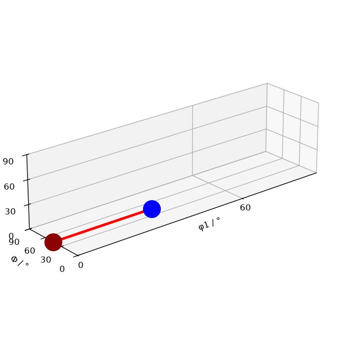
Plotting the Endpoint Segment

The default three-dimensional plot uses Bunge Euler coordinates.

plot(f, lineWidth=3, lineColor='red')
hold(True)
plot(oriA, filled=True, markerSize=20, markerFaceColor='darkred')
plot(oriB, filled=True, markerSize=20, markerFaceColor='blue')
plt.xlim(0, 90)
hold(False)

Reading the Endpoint Plot

The red segment joins the dark-red Goss endpoint at \((0,45,0)\) degrees to the blue Brass endpoint at \((35,45,0)\) degrees. Only the first Euler angle changes in this example, so the segment looks straight. In general, angular distance is not Euclidean distance in an Euler coordinate plot.

The Two Directions That Define a Fibre

An orientation maps a direction from the crystal frame into the specimen frame. Every orientation ori on the full fibre satisfies

The endpoint constructor has already computed these directions. They are available as the h and r properties of fibre.

h = f.h
h

vector3d (432)
  u       v       w
  0  0.7071  0.7071

r = f.r
r

vector3d (y↑→x)
  x  y  z
  0  0  1

Both endpoints map h exactly onto r. The two displayed entries are their mapping errors in degrees.

mappingErrorDegrees = np.array([angle(oriA * h, r), angle(oriB * h, r)]) / degree
mappingErrorDegrees

array([0., 0.])

A Full Fibre

The option full=True discards the finite endpoint and continues the curve through every rotation about the aligned direction.

fullFibre = fibre(oriA, oriB, full=True)
fullFibre

fibre (432 → y↑→x)
  h || r: [011] || (0,0,1)

A crystal–specimen direction pair constructs the same full fibre directly. The displayed logical value confirms that the two definitions agree.

directionFibre = fibre(h, r)
sameFullFibre = fullFibre.isclose(directionFibre)
sameFullFibre

True

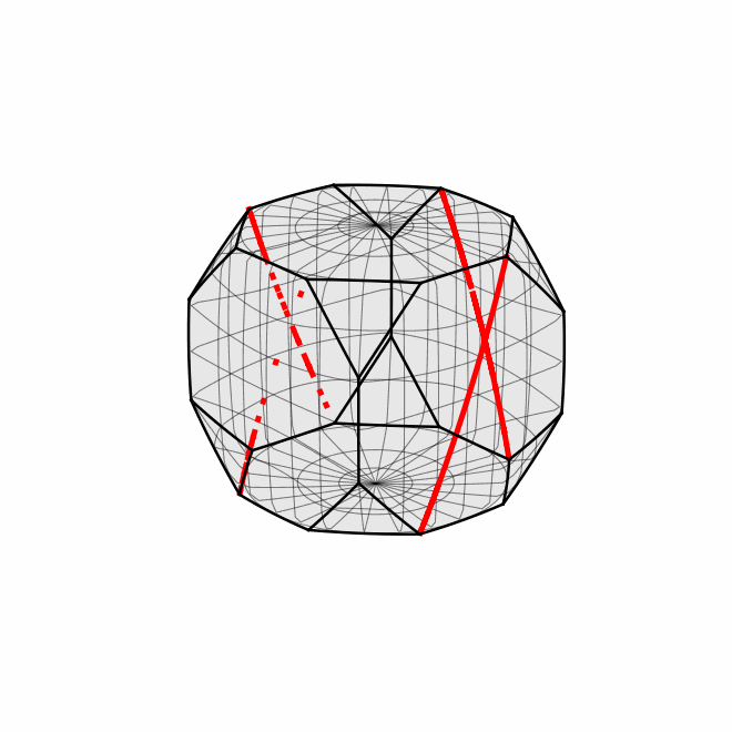
Symmetry Can Split the Plot

By default, an orientation plot is folded into a fundamental region.

plot(fullFibre, 'axisAngle', lineWidth=3, lineColor='red')
plt.gca().set_axis_off()

Reading the Symmetry-Reduced Plot

The red fibre appears as disconnected arcs because it leaves the chosen fundamental region and re-enters through a symmetry-equivalent face. These arcs belong to one fibre, not to several different fibres.

The Complete Axis–Angle Domain

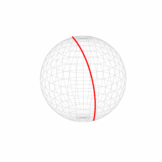
The option complete=True removes the reduction by crystal symmetry.

plot(fullFibre, 'axisAngle', complete=True, lineWidth=3, lineColor='red')
plt.gca().set_axis_off()

Reading the Complete Plot

The complete axis–angle ball exposes more of the red curve without the cubic fundamental-region faces. It still has a coordinate seam: opposite points on the outer sphere describe the same half turn. A curve cut at that seam is therefore still one closed fibre in rotation space.

Sampling a Fibre

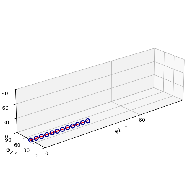
orientation discretises a fibre for plotting or numerical calculations. Specify the number of samples when it matters.

sampledOri = orientation(f, points=12)
numberOfSamples = len(sampledOri)
numberOfSamples

12

The markers show the 12 sampled orientations on the finite endpoint segment. The continuous red curve remains the underlying fibre.

plot(f, lineWidth=2, lineColor='red')
plt.xlim(0, 90)
hold(True)
plot(sampledOri, markerSize=8, markerEdgeColor='darkblue', lineWidth=2)
hold(False)

Why a Full Fibre Is a Circle

Unit quaternions represent rotations with the identification \(q=-q\). Starting from a quaternion \(q_0\), a spin through the angle \(\omega\) about the aligned direction traces

As \(\omega\) runs from 0 to \(2\pi\), this path follows half of a great circle on the unit 3-sphere from \(q_0\) to \(-q_0\). Those endpoints represent the same rotation, so their projection into rotation space is a closed circle. The finite fibre constructed first is one subarc of this circle.

Where Fibres Reappear in MTEX

angle measures the distance from an orientation to a fibre. Fibres of Orientations develops pole-figure and inverse-pole-figure plots, symmetrisation, and named rolling-texture fibres. Fibre ODFs spreads a density around a fibre.

Pole-figure values integrate an ODF over fibres. This integration is the crystallographic Radon transform developed in the pole figure tutorial.

Further Reading

• A. Morawiec, Orientations and Rotations: Computations in Crystallographic Textures, Springer, 2004, develops the geometry of rotation space and its symmetry-reduced regions.
• H.-J. Bunge, Texture Analysis in Materials Science: Mathematical Methods, Butterworths, 1982, develops fibre textures and orientation distributions.
• D. Chateigner, L. Lutterotti and M. Morales, Quantitative texture analysis and combined analysis, International Tables for Crystallography, Volume H, 2019, places fibre textures and the Radon transform in diffraction texture analysis.

Next

Continue with Fibres of Orientations for crystallographic plotting and named texture fibres, then Fibre ODFs for density models around them.

Technical Details

A fibre stores its two orientations and the aligned direction; h, r and the arc are derived. full=True is MATLAB’s 'full' flag, orientation(f, points=12) samples it.

@article{bachmann2010mtex,
  author  = {F. Bachmann and R. Hielscher and H. Schaeben},
  title   = {Texture Analysis with MTEX - Free and Open Source Software Toolbox},
  journal = {Solid State Phenomena},
  volume  = {160},
  pages   = {63-68},
  year    = {2010},
  doi     = {10.4028/www.scientific.net/SSP.160.63},
  url     = {https://doi.org/10.4028/www.scientific.net/SSP.160.63}
}