The sphericity as measure for grain boundary irregularity
Deformed polycrystalline materials such as ice often contain large grains interlocking with smaller grains, with many irregular grain boundaries. Boundary irregularity is hard to judge by visual inspection and it is better to use quantitative measures of boundary irregularity to infer processes across different deformation conditions. Here, we quantify the irregularity of each grain’s boundary by introducing a sphericity parameter \(\Psi\) which is calculated in 2-D from grain area A, grain boundary perimeter P, and area equivalent grain radius R by the formula
\[\Psi = \frac{A}{P \cdot R}\]
The grain sphericity \(\Psi\) is a useful indicator for grain boundary irregularity because it measures how closely a grain’s boundary resembles the circumference of a perfect circle. It decreases from \(\Psi = 0.5\), where the grain has a perfect circular shape, to \(\Psi = 0\) where the grain boundary is infinitely irregular. The statistics of grain boundary sphericity can be used to segregate recrystallised grains from remnant original grains (please refer to the paper for more details).
Data
The EBSD data set used in this demonstration (PIL185.ctf) is available from https://doi.org/10.6084/m9.figshare.13456550. The EBSD data were collected with a step size of 5 µm and representeds an ice sample deformed at -20°C to 12 percent axial strain. Let's import the data and reconstruct some grains.
% plotting convention
plotx2east
plotzIntoPlane

% import the data
path = [mtexExamplePath filesep 'GrainExamples' filesep ];
ebsd = EBSD.load([path 'PIL185.ctf'],'convertSpatial2EulerReferenceFrame');

% critical misorientation for grain reconstruction
threshold = 10 *degree;

% first pass at reconstructing grains
[grains, ebsd.grainId] = calcGrains(ebsd('ice'),'angle',threshold);

% remove ebsd data that correspond to up to 4 pixel grains
ebsd(grains(grains.grainSize < 5)) = [];

% redo grain reconstruction - interpolate non-indexed space
[grains, ebsd.grainId] = calcGrains(ebsd('ice'),'angle',threshold);

% remove all boundary grains
grains(grains.isBoundary) = [];

% remove too small irregular grains
grains(grains.grainSize < grains.boundarySize / 2) = [];

% plot the result
plot(ebsd,ebsd.orientations)

hold on
plot(grains.boundary)
hold off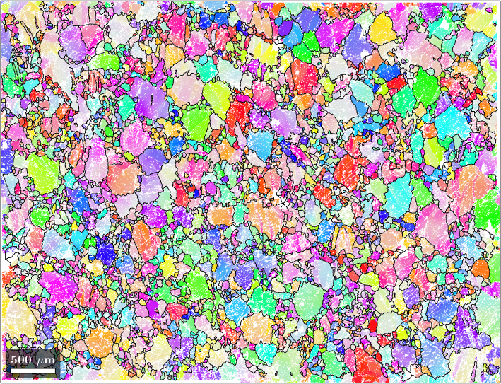
Computation of the Sphericity
Next, let's calculate and plot the sphericity parameter of each ice grain by making use of the functions grains.area, grains.perimeter and grains.equivalentRadius
% directly use the formula from the first paragraph
Psi = grains.area ./ grains.perimeter('withInclusion') ./ grains.equivalentRadius;

% plot the result
plot(grains, Psi, 'colorrange', [0 0.5])

mtexColorbar ('title','Sphericity Parameter')
mtexColorMap jet
clear Psi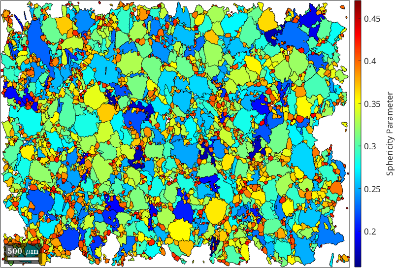
Influence of EBSD step size on sphericity parameter
Next we investigate how step size influences grain boundary irregularity measurements. To do this, we can artificially increase the step size of the EBSD data to from 10 up to 100 μm. Then, we choose one representative grain (one with a large number of pixels) and see how the sphericity parameter changes as the EBSD step size increases.
newMtexFigure('layout',[4,5])
for i = 1:20

  % now, we increase the step size of EBSD data artifically
  ebsd_reduced = reduce(ebsd,i);

  % reconstruct grains using function calcGrains
  grains_reduced = calcGrains(ebsd_reduced('ice'));

  % choose a grain with a large pixel number within the EBSD map with 5
  % micron step size, from each reduced EBSD map by location
  grain = grains_reduced(findByLocation(grains_reduced('ice'), [1357 1952]));

  % calculate the sphericity parameter
  Psi(i) = grain.area ./ (grain.perimeter('withInclusion') .* grain.equivalentRadius);

  % calculate the number of pixels
  gS(i) = grain.grainSize;

  % plot evolution of grain geometry as step size increases
  if i>1, nextAxis; end
  plot(grain, Psi(i),'doNotDraw','micronbar','off')
  mtexTitle([int2str(5*i) '\(\mu\)m'],'doNotDraw');

end

setColorRange([0 0.5])
mtexColorMap jet
mtexColorbar ('title', 'sphericity parameter')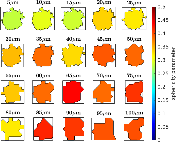
Now we are able to plot the sphericity parameter as a function of the step size.
clf
scatter (gS, Psi, 150,5:5:100,'filled','MarkerEdgeColor','k','linewidth', 1.5)
colormap gray

C = colorbar;
C.Label.String = 'EBSD step size, \mum';
C.Ticks = 5:10:100;
xlabel('LOG (number of pixels)')
ylabel('Sphericity parameter')
set (gca, 'xscale', 'log')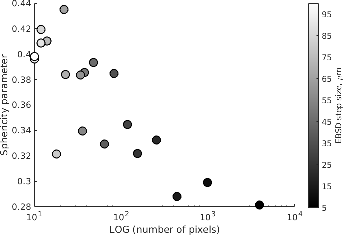
Influence of grain boundary smoothness on sphericity parameter
Due to the square shape of pixels (prescribed by Oxford Instruments software), boundary elements lie either vertically or horizontally within the plane of analysis. Grains containing fewer pixels (i.e., smaller grains in maps with a fixed step size) appear more pixelated than grains containing numerous pixels. MTEX allows us to reduce artificial pixelation of grain boundary elements by applying the function smooth, which enhances the overall grain boundary smoothness by interpolating the coordinates of grain boundary elements while triple junction points remain locked or unlocked. In this study, we choose to lock the triple junction during grain boundary smoothening.
newMtexFigure('layout',[3,3],'figSize','normal');

% find all grains with more than 2000 pixels
grains = grains(grains.grainSize > 2000);

for m = 1:36

  % Smooth grain boundary to reduce pixelation, a larger m (smoothening
  % parameter corresponds to a greater grain boundary smoothening
  smoothGrains = smooth(grains, m);

  % calculate the sphericity parameter for smoothed grains
  Psi(m) = median(smoothGrains.area ./ smoothGrains.equivalentRadius ./ smoothGrains.perimeter('withInclusion') );

  if mod(m,4)~=1, continue; end

  % Visualise the evolution of grain boundary geometry as the smoothening
  % parameter increases, using a grain as an example

  % select grain
  grain = smoothGrains(findByLocation(smoothGrains, [1357 1952]));

  % plot it
  if m>1, nextAxis; end
  plot(grain, grain.area ./ grain.equivalentRadius ./ grain.perimeter('withInclusion'),...
    'micronbar','off','doNotDraw');
  mtexTitle(['m=',int2str(m)],'doNotDraw');

end

setColorRange([0 0.5])
mtexColorbar jet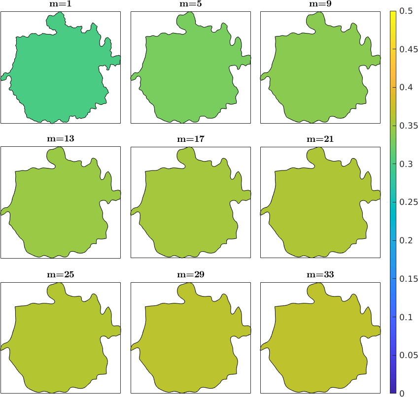
Finally we plot the sphericity as a function of the smoothening parameter
clf
plot(1:length(Psi), Psi, 'o')
xlabel ('Smooth parameter')
ylabel ('Sphericity parameter')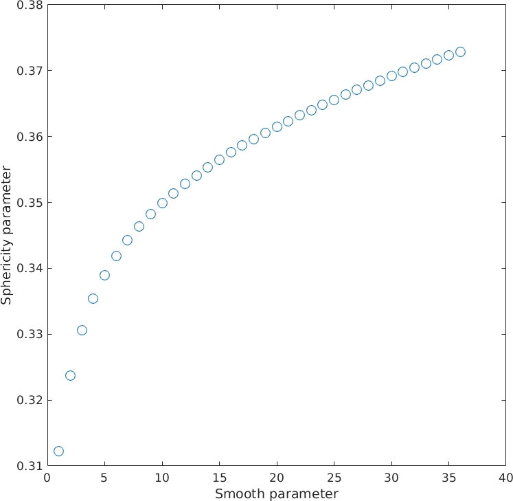
References
- Sheng Fan, David J. Prior, Andrew J. Cross, David L. Goldsby, Travis F. Hager, Marianne Negrini, Chao Qi, Using grain boundary irregularity to quantify dynamic recrystallization in ice, Acta Materialia, 2021.