Harmonic Approximation from Discrete Data

Approximating Orientation-Dependent Functions from Discrete Data defines the approximation problem and compares the available models. This page assumes that a harmonic model is appropriate and shows how to control its bandwidth, regularisation, sample weights, and iterative solver.

Harmonic approximation is particularly useful for a general physical response that is not a density function. It also handles large numbers of sample orientations without placing one kernel at every observation. Noisy experimental data should be approximated rather than interpolated exactly, because an exact fit would reproduce the noise.

A noisy data set

Start with the same orientation-dependent data as on the overview page. The standard deviation of the added noise is 5 percent of the standard deviation of the supplied values.

import numpy as np

from mtex import *

rng = np.random.default_rng(1)
fname = mtexdatafile('dubnaValues')
ori, S = loadOrientation(fname, columnNames=['phi1', 'Phi', 'phi2', 'values'])
val = S['values'] + rng.standard_normal(S['values'].shape) * 0.05 * np.std(S['values'], ddof=1)

plotSection(ori, val, 'sigma', all=True)

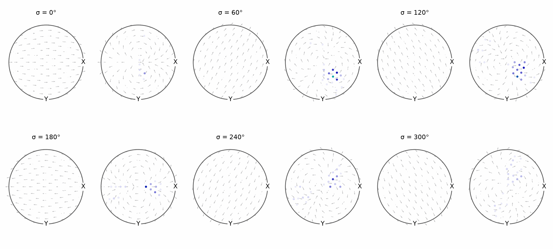
The strongest regions still occupy the same sections as in the original data, but neighbouring markers now fluctuate. A fitted surface should recover the broad regions without chasing those point-to-point changes.

Start with bandwidth

interp selects a harmonic fit with the flag 'harmonic'. Internally it calls SO3FunHarmonic.interpolate. The bandwidth is the largest harmonic degree in the fitted series. A low bandwidth limits the number of unknown coefficients and therefore limits how quickly the function can vary.

Set regularisation to zero temporarily so that the effect of bandwidth is visible on its own.

SO3F1 = interp(ori, val, 'harmonic', regularisation=0, bandwidth=17)
SO3F1

SO3FunHarmonic (1 → y↓→x)
  bandwidth: 17
  mean     : 0.9938

numberOfSamples = ori.size
numberOfSamples

10432

numberOfCoefficients17 = SO3F1.fhat.size
numberOfCoefficients17

7770

relativeError17 = norm(SO3F1.eval(ori) - val) / norm(val)
relativeError17

0.0754

plot(SO3F1, 'sigma')

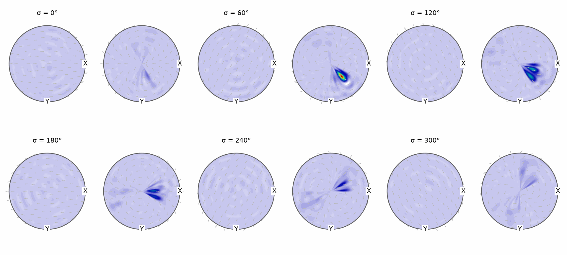
There are more samples than coefficients in this bandwidth-17 fit, so the least-squares system is overdetermined. The fit is smooth and does not pass through every noisy sample. Its nonzero residual is expected, not a defect.

Raising the bandwidth to 32 introduces more coefficients than samples. This makes the system underdetermined. It is the opposite of oversampling: oversampling means having more independent samples than unknowns.

SO3F2 = interp(ori, val, 'harmonic', regularisation=0, bandwidth=32)
SO3F2

SO3FunHarmonic (1 → y↓→x)
  bandwidth: 32
  mean     : 0.2474

numberOfCoefficients32 = SO3F2.fhat.size
numberOfCoefficients32

47905

relativeError32 = norm(SO3F2.eval(ori) - val) / norm(val)
relativeError32

4.1064e-04

plot(SO3F2, 'sigma')

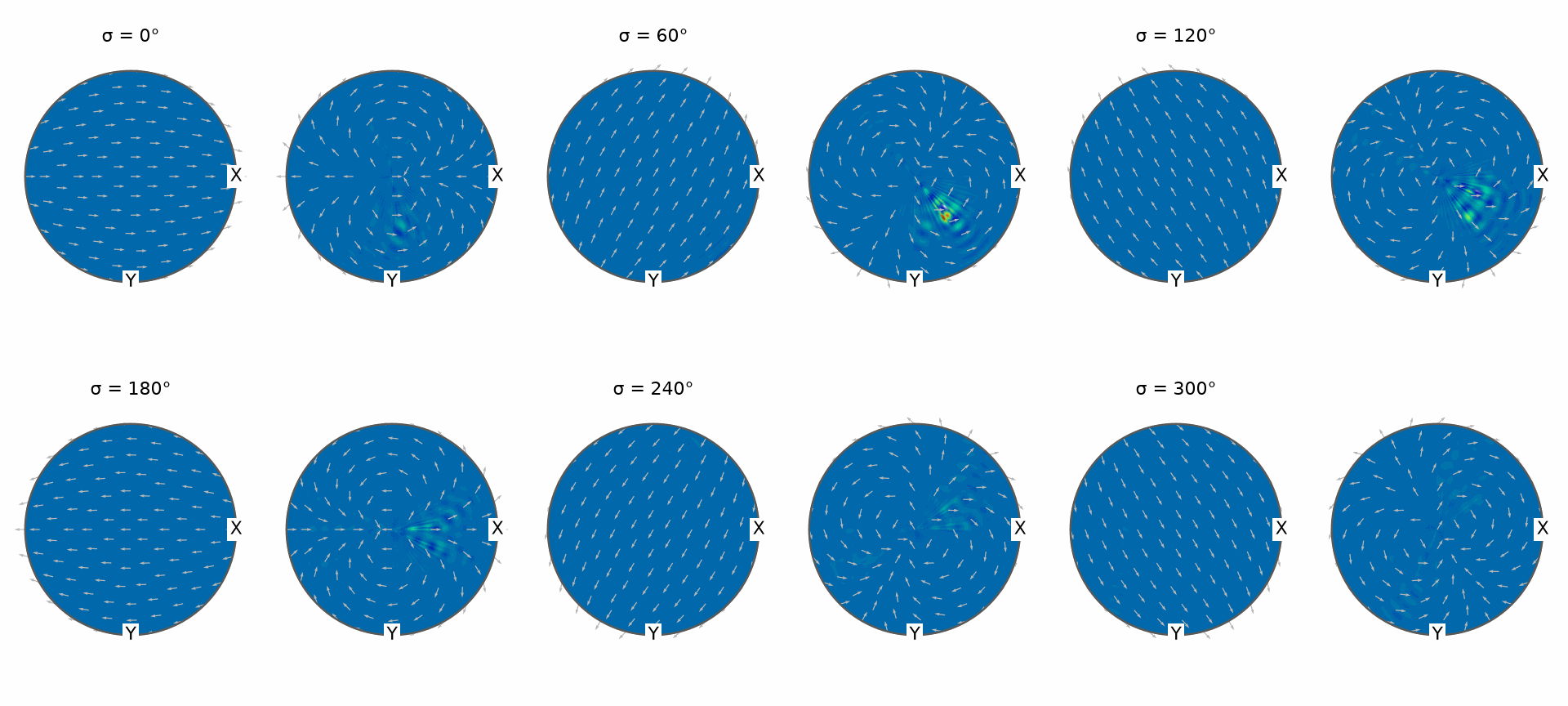
The higher-bandwidth surface follows the samples more closely, so its residual is smaller. The narrow peaks and alternating ripples between them are evidence of overfitting. If LSQR reaches its iteration limit, treat the displayed residual as an unconverged value rather than the optimum of the least-squares problem.

Read the spectrum

plotSpectrum summarizes the coefficient energy at each harmonic degree. It reveals high-frequency content that can be difficult to distinguish in a section plot.

plotSpectrum([SO3F1, SO3F2], figSize='small')
legend('Bandwidth 17', 'Bandwidth 32')

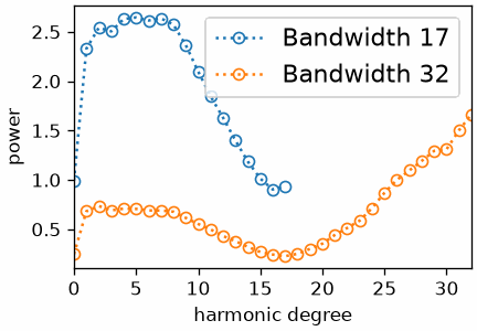
The bandwidth-17 spectrum stops before the high degrees are available. For bandwidth 32, the energy fails to decay towards the cutoff and even increases at high degrees. That high-degree tail matches the oscillations in the preceding section plot and is a practical overfitting diagnostic.

Add regularisation

Tikhonov regularisation penalizes high-degree coefficient energy. It lets you retain a bandwidth high enough for sharp real features while making oscillatory solutions more expensive.

Current MTEX uses \(\lambda=10^{-8}\) by default and a Sobolev index \(s=2\). Older versions of this example documented \(5\mathbin{\cdot}10^{-7}\) as the default. That value is retained here as an explicit smoothing choice, not as the current default. A suitable value depends on the data and should be checked rather than accepted automatically.

SO3F3 = interp(ori, val, 'harmonic', bandwidth=32, regularisation=5e-7)
relativeErrorReg = norm(SO3F3.eval(ori) - val) / norm(val)
relativeErrorReg

0.0062

plot(SO3F3, 'sigma')

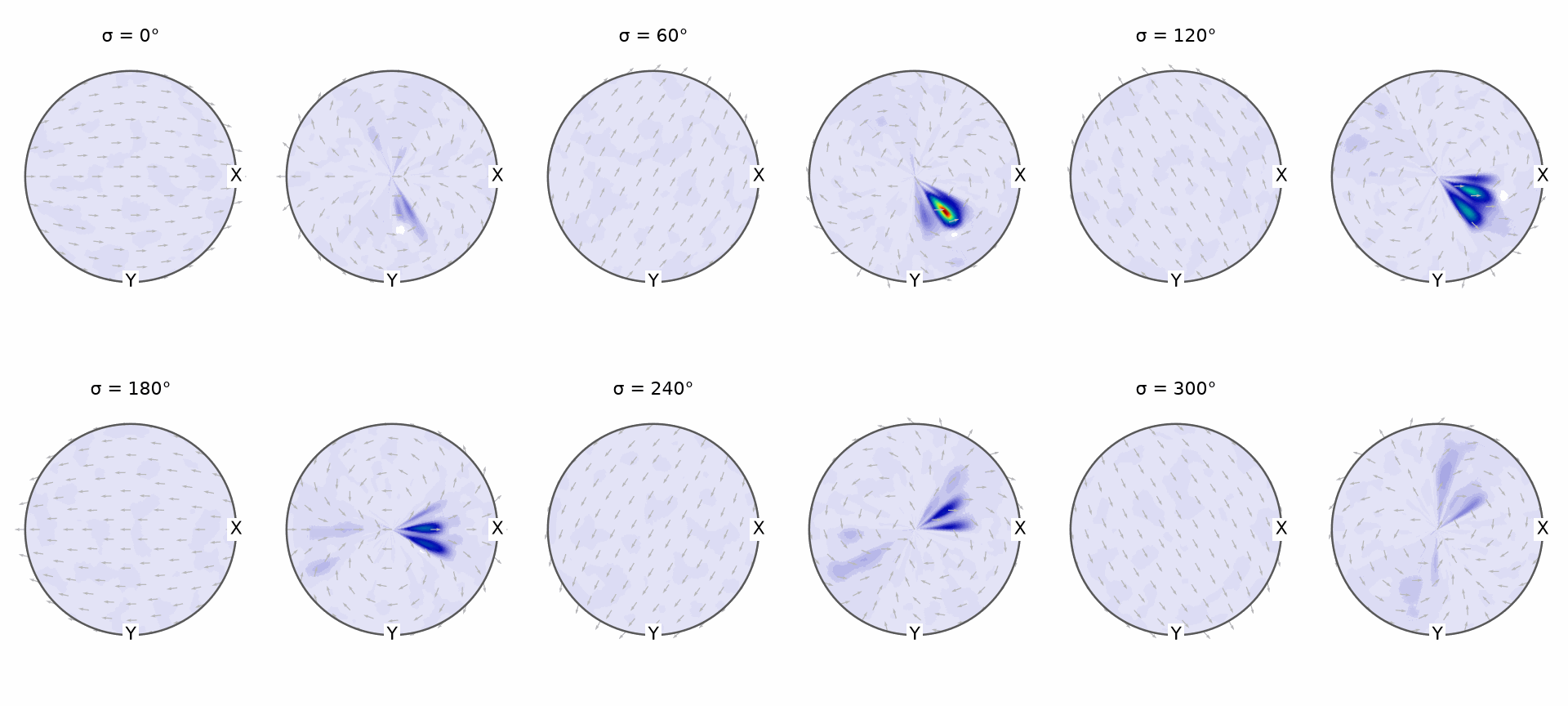
The bandwidth remains 32, but the unsupported narrow peaks are suppressed. The residual at the noisy samples is larger because the fit now balances agreement with smoothness. That residual is only the data term; it is not the complete regularized objective minimized by LSQR.

Sweep the regularisation parameter

A very large \(\lambda\) drives the fitted function towards zero. A very small value approaches the unregularized, oscillatory solution. The sweep below spans both failures so that the useful transition can be seen.

reg = [1, 1e-1, 1e-2, 1e-3, 1e-4, 1e-5, 1e-6, 1e-7, 1e-8, 1e-9, 1e-10, 1e-11, 1e-12, 1e-13, 1e-14]
SO3F4 = [interp(ori, val, 'harmonic', bandwidth=32, regularisation=r) for r in reg]

newMtexFigure(layout=[5, 6])
for i, r in enumerate(reg):
  if i > 0:
    nextAxis()
  plot(SO3F4[i], 'sigma', 0 * degree)
  legend(f'λ = {r:g}')
setColorRange('tight')
mtexColorbar()

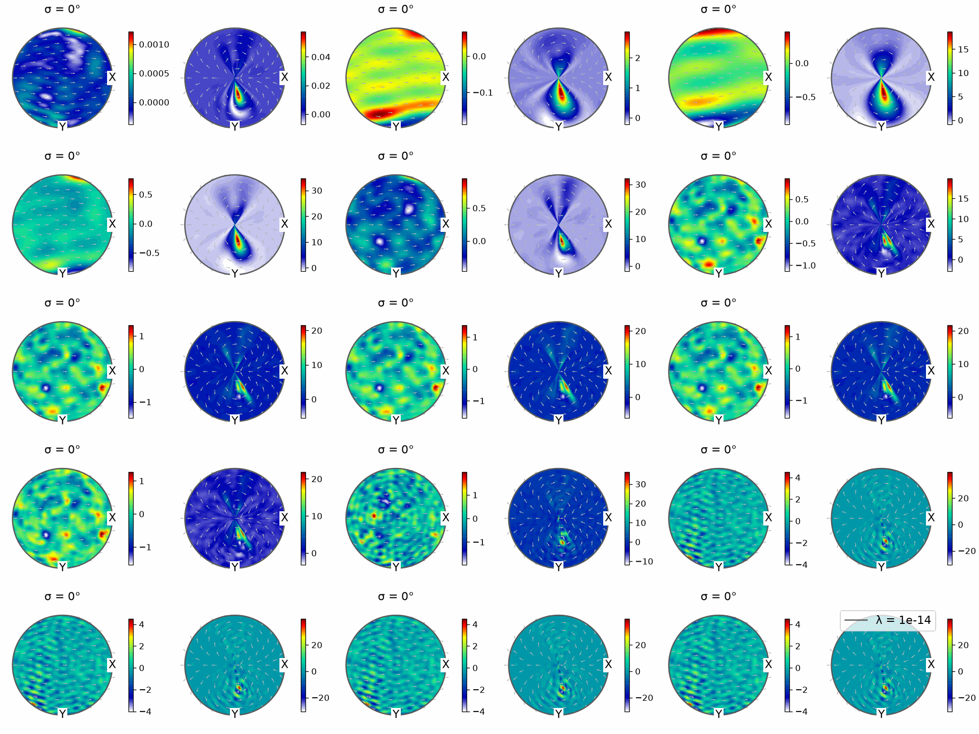
Every section of a function without crystal symmetry is a pair of discs, the upper and the lower hemisphere. Read the pairs from left to right and top to bottom as \(\lambda\) decreases. The first panels are almost zero because the penalty dominates. Structure appears at intermediate values. At the smallest values, sharp fluctuations return because agreement with the noisy samples dominates.

The corresponding spectra make that transition quantitative. The selected indices represent \(\lambda=10^{-2}\), \(10^{-4}\), \(10^{-8}\), and \(10^{-12}\).

ind = [2, 4, 8, 12]
plotSpectrum([SO3F4[i] for i in ind], figSize='small')
legend('λ = 10⁻²', 'λ = 10⁻⁴', 'λ = 10⁻⁸', 'λ = 10⁻¹²')

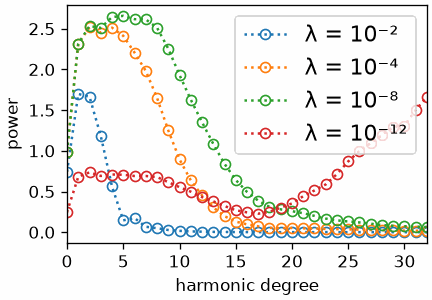
Strong regularisation removes almost all high-degree energy. As \(\lambda\) decreases, the tail rises. Choose a value before the tail becomes dominated by high-degree energy, then confirm the choice against held-out data or independent physical expectations.

Change the Sobolev index

The Sobolev index controls how quickly the penalty grows with harmonic degree. A smaller index penalizes high degrees less strongly. The value of \(\lambda\) must therefore be reconsidered whenever \(s\) changes.

SO3F5 = interp(ori, val, 'harmonic', bandwidth=32, regularisation=0.001, SobolevIndex=1)
SO3F5

SO3FunHarmonic (1 → y↓→x)
  bandwidth: 32
  mean     : 0.992

newMtexFigure(layout=[1, 4])
plot(SO3F4[3], 'sigma', 0 * degree)
legend('s = 2')
nextAxis()
plot(SO3F5, 'sigma', 0 * degree)
legend('s = 1')
setColorRange('equal')
mtexColorbar()

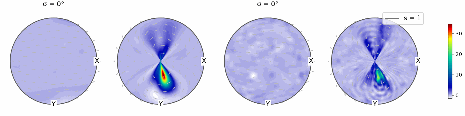
Both pairs use \(\lambda=0.001\). The \(s=1\) panel retains more fine-scale variation because its high-degree penalty grows more slowly. Matching \(\lambda\) numerically does not mean that the two fits have equal smoothing.

Weight nonuniform or unequal samples

Weighted least squares controls how strongly each sample contributes to the data residual. Use weights='equal' when every observation should count equally. Use weights='Voronoi' to compensate for nonuniform sampling by orientation-space cell volume, or pass one numeric weight per sample when measurement uncertainties are known.

MTEX computes Voronoi weights by default for fewer than 10,000 samples. It uses equal weights for larger sets because the Voronoi calculation is time-consuming. This data set has slightly more than that threshold, so its default weights are equal. The explicit forms are:

SO3F = interp(ori, val, 'harmonic', weights='equal')
SO3F = interp(ori, val, 'harmonic', weights='Voronoi')
SO3F = interp(ori, val, 'harmonic', weights=measurementWeights)

Numeric weights describe relative confidence or integration volume. They do not impose nonnegativity and do not turn a harmonic fit into a density.

Control LSQR convergence

LSQR stops when it reaches its tolerance tol or iteration limit maxIter. Their defaults are 1e-3 and 100. A smaller tolerance requests a more accurate iterative solution, but the iteration limit may stop the solver first. Premature stopping can itself have a regularizing effect, so it must not be confused with convergence.

With withParameters=True the direct interpolation method also returns the LSQR diagnostics. The first entry is the exit flag, the second the relative residual, and the third the number of iterations.

f1, p1 = SO3FunHarmonic.interpolate(ori, val, withParameters=True)
print(f'default: flag {p1[0]}, relative residual {p1[1]:.6g}, iterations {p1[2]}')

f2, p2 = SO3FunHarmonic.interpolate(ori, val, tol=1e-15, withParameters=True)
print(f'tight tol: flag {p2[0]}, relative residual {p2[1]:.6g}, iterations {p2[2]}')

default: flag 0, relative residual 0.0509289, iterations 37
tight tol: flag 1, relative residual 0.0509115, iterations 100

Compare the flags before comparing the residuals. If the tight-tolerance run stops at 100 iterations, increase maxIter deliberately and check whether the fit and validation error materially change.

Earlier code on this page printed norm(f.eval(ori)-val)+5e-7*norm(f,2) as the “energy functional”. That expression is not the minimized objective: it omits the squared norms, uses a fixed historical \(\lambda\), and does not reproduce the coefficient weights used internally.

The maths behind harmonic approximation

A bandlimited harmonic function is a finite series of Wigner-D functions:

The coefficient vector \(\mathbf{\hat f}\) is chosen to minimize the data residual at the \(M\) sample pairs \((x_m,v_m)\). Without regularisation, the problem is

With Tikhonov regularisation, MTEX minimizes

where the implemented Sobolev penalty is

Larger \(s\) increases the relative cost of high-degree coefficients. Larger \(\lambda\) increases the overall influence of that cost.

The Fourier matrix has entries \(F_{m,(n,k,l)}=D_n^{k,l}(x_m)\). MTEX does not need to form this dense matrix explicitly. LSQR repeatedly applies the matrix and its adjoint, and MTEX evaluates those products with Wigner transforms and the nonequispaced fast Fourier transform (NFFT). This is why lowering bandwidth reduces the number of unknowns and the computational cost; it does not make the mathematical Fourier matrix sparse.

References

• C. C. Paige and M. A. Saunders, LSQR: An algorithm for sparse linear equations and sparse least squares, ACM Transactions on Mathematical Software 8 (1982), 43-71, introduces the iterative solver and its convergence diagnostics.
• J. Keiner, S. Kunis, and D. Potts, Using NFFT 3: A software library for various nonequispaced fast Fourier transforms, ACM Transactions on Mathematical Software 36 (2009), Article 19, describes the transforms used for fast matrix-vector products at nonequispaced orientations.

Next

Continue with RBF-Kernel Interpolation to replace the global harmonic series by local kernels and to compare the available constrained and unconstrained least-squares solvers.

Technical Details

MATLAB’s second output of SO3FunHarmonic.interpolate is withParameters=True here, the flag, the relative residual and the iterations of LSQR; the noise is drawn by NumPy. MATLAB’s LSQR evaluates the series at the nodes through an NFSOFT of cutoff parameter 1, not the accurate one: on the noise-free values and \(\lambda=5\mathbin{\cdot}10^{-7}\) its fit misses the data by 0.051 under that transform, the port’s by 0.053, but evaluated accurately MATLAB’s misses it by 0.206. The port’s transforms are exact, so its residuals of the bandwidth-32 fits, 0.0013 and 0.0062, are the ones of the least-squares problem where MATLAB reports 0.0159 and 0.0239. MATLAB draws a sigma section of a triclinic function on the upper hemisphere only, since it takes the plane normal \(c^*\) as antipodal and so equivalent to \(-c^*\); that hides half of the orientations, among them the peak of the Dubna data. The port draws both hemispheres, so a section is a pair of discs and the layouts have twice MATLAB’s columns.

@article{bachmann2010mtex,
  author  = {F. Bachmann and R. Hielscher and H. Schaeben},
  title   = {Texture Analysis with MTEX - Free and Open Source Software Toolbox},
  journal = {Solid State Phenomena},
  volume  = {160},
  pages   = {63-68},
  year    = {2010},
  doi     = {10.4028/www.scientific.net/SSP.160.63},
  url     = {https://doi.org/10.4028/www.scientific.net/SSP.160.63}
}