Approximating Orientation-Dependent Functions from Discrete Data

Suppose that a quantity has been measured at orientations \(\mathtt{ori}_m\), with one value \(v_m\) at each orientation. The task is to replace those samples by a function that can be evaluated and plotted at any orientation. MTEX calls this operation interp, although the fitted function need not pass through every sample exactly.

The values may be an orientation distribution function (ODF), such as volume fractions measured at different orientations. They may instead be any scalar physical property that depends on orientation. This distinction determines whether the fitted function must be nonnegative and have mean 1.

import numpy as np

from mtex import *

plottingConvention.default('y↑→x')

Importing the samples

An ASCII file can contain one orientation and one or more measured values per row. loadOrientation needs the columns of the Euler angles and the names of the additional columns.

fname = mtexdatafile('dubnaValues')
ori, S = loadOrientation(fname, columnNames=['phi1', 'Phi', 'phi2', 'values'])

The result ori contains the sample orientations. The table S has one column for every additional column of the file, so the values in this file are available as S['values'].

plotSection(ori, S['values'], 'sigma', all=True)

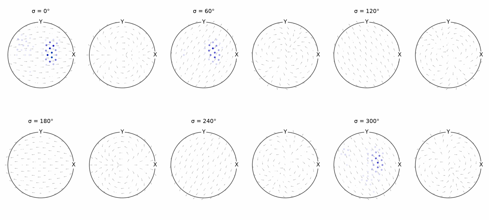
Each marker in the section plot is one sample, and its colour is the corresponding value. Notice the isolated high-value regions and the large areas with values close to zero. A useful approximation should retain those regions without introducing unsupported oscillations.

Choosing an approximation

Approximation finds a function that agrees reasonably well with the data. Interpolation is the special case in which it agrees exactly at the sample orientations. Noise, incomplete sampling, or regularisation often makes approximation the more useful goal.

interp provides three approximation schemes:

• A harmonic expansion is a global series model. Prefer it for a general orientation-dependent relationship, especially with many nodes, outliers, or noise.
• A radial-basis-function (RBF) model is a weighted sum of kernels centred on a grid. Prefer it for an ODF with a low or medium number of nodes, and use 'density' when nonnegativity and mean 1 are required.
• A Bingham distribution is a compact parametric density model. Use it only when one Bingham-shaped component is physically appropriate.

These are starting points rather than rules. In practice, compare the computational cost and the fitted shapes from both harmonic and RBF models. The residual at the samples is useful, but it cannot by itself reveal oscillations or overfitting between them.

Harmonic approximation

The flag 'harmonic' selects a harmonic expansion. Internally, interp calls SO3FunHarmonic.interpolate. The default fit includes regularisation, which suppresses rapidly varying harmonic coefficients.

SO3FReg = interp(ori, S['values'], 'harmonic')
SO3FReg

SO3FunHarmonic (1 → y↑→x)
  bandwidth: 18
  mean     : 0.9974

relativeErrorReg = norm(SO3FReg.eval(ori) - S['values']) / norm(S['values'])
relativeErrorReg

0.0463

plot(SO3FReg, 'sigma')

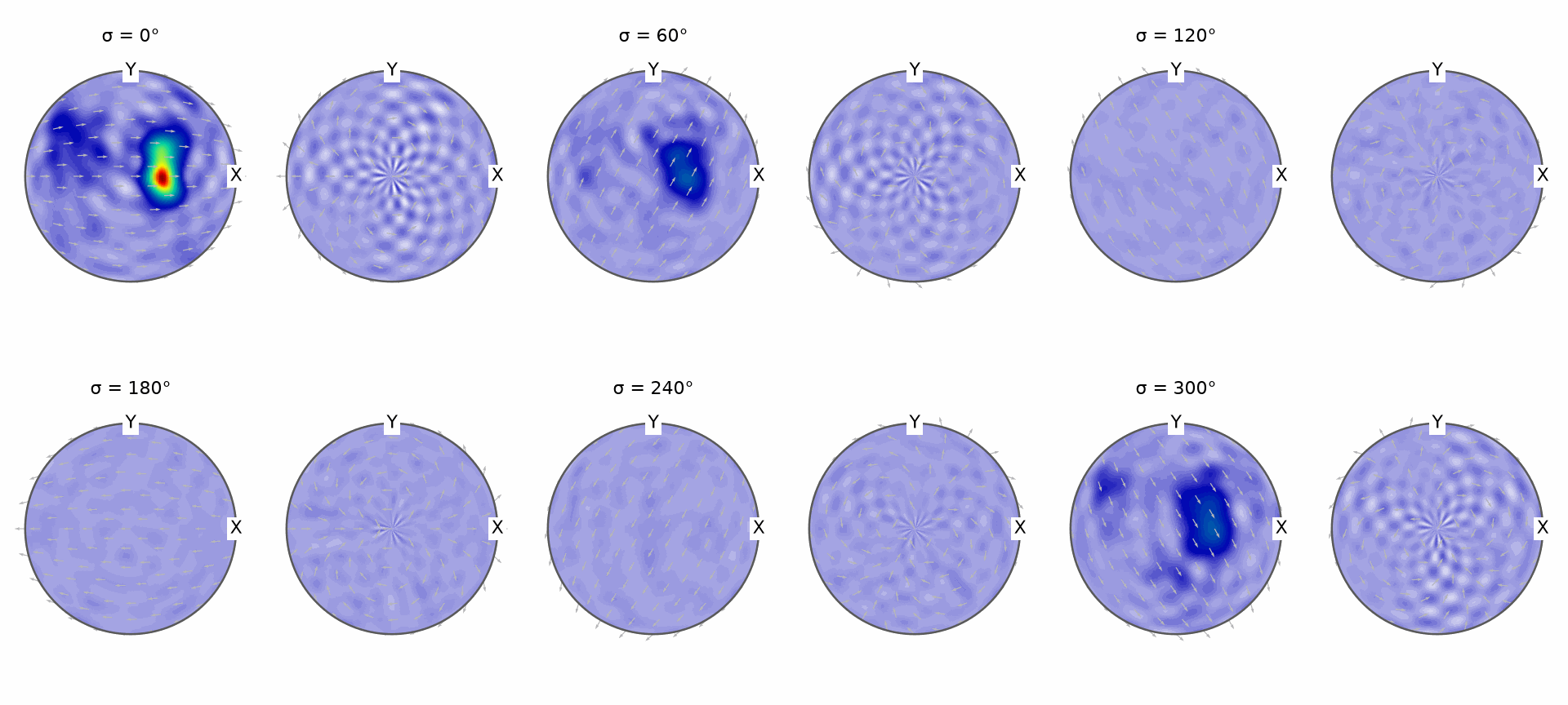
Compare this plot with the discrete samples. The strongest regions remain in the same sections, while regularisation rounds their peaks and prevents the fit from following every local variation.

The default regularisation parameter is \(\lambda=10^{-8}\). Setting it to zero switches regularisation off and asks the harmonic model to follow the samples more closely.

SO3FUnreg = interp(ori, S['values'], 'harmonic', regularisation=0)
SO3FUnreg

SO3FunHarmonic (1 → y↑→x)
  bandwidth: 18
  mean     : 0.9973

relativeErrorUnreg = norm(SO3FUnreg.eval(ori) - S['values']) / norm(S['values'])
relativeErrorUnreg

0.0463

plot(SO3FUnreg, 'sigma')

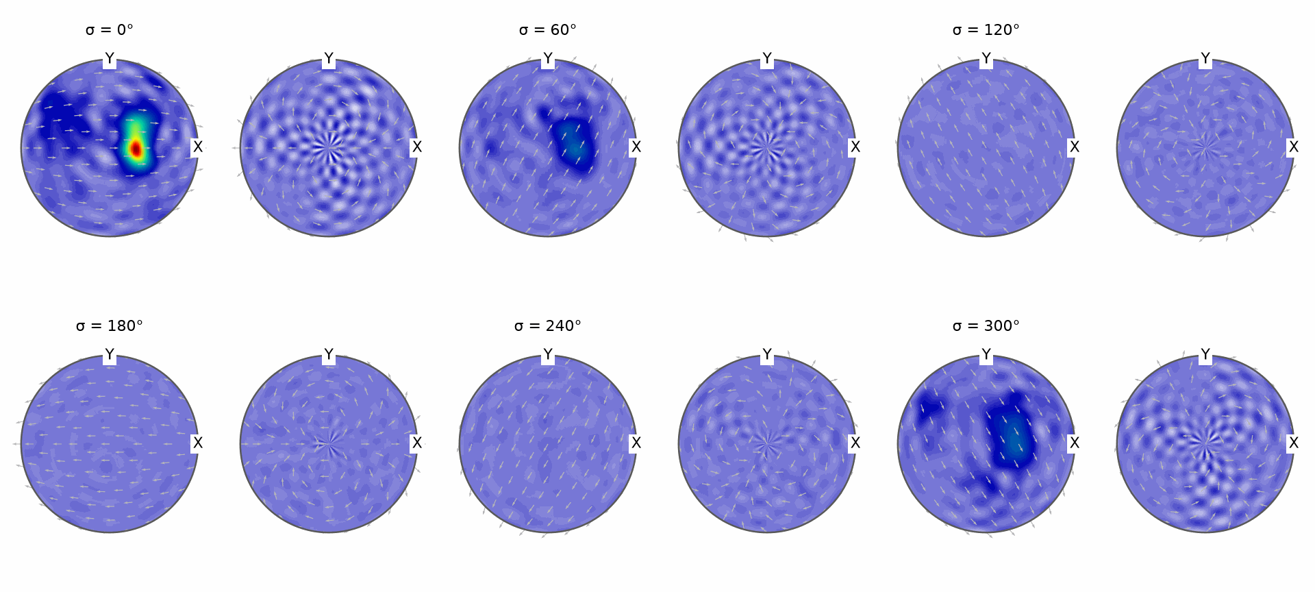
A converged unregularized solution is free to make the residual much smaller, but it can create narrow peaks and ripples between the samples. Do not interpret an unconverged residual as the optimum. Even after convergence, a smaller residual is not by itself evidence for a better model. The next page explains how to choose regularisation and check solver convergence.

Reducing the harmonic bandwidth is another form of regularisation. The bandwidth is the largest harmonic degree retained by the series.

SO3FLow = interp(ori, S['values'], 'harmonic', regularisation=0, bandwidth=16)
SO3FLow

SO3FunHarmonic (1 → y↑→x)
  bandwidth: 16
  mean     : 0.9981

relativeErrorLow = norm(SO3FLow.eval(ori) - S['values']) / norm(S['values'])
relativeErrorLow

0.1057

plot(SO3FLow, 'sigma')

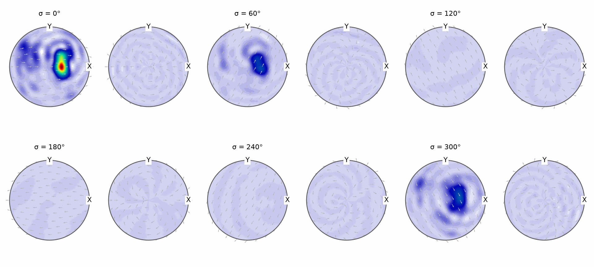
The bandwidth-16 fit cannot reproduce variations finer than its truncated series permits. It is smoother than the unrestricted unregularized fit, but bandwidth alone does not enforce the physical constraints of an ODF. In particular, harmonic approximation cannot guarantee a nonnegative function even when every supplied value is nonnegative.

minimumHarmonicValue = min(SO3FLow)[0]
minimumHarmonicValue

-12.2598

Density-constrained RBF approximation

Without a method flag, interp uses an RBF model and internally calls SO3FunRBF.interpolate. The 'density' flag constrains the weights so that the result is nonnegative and then normalizes its mean to 1.

SO3FDensity = interp(ori, S['values'], density=True)
relativeErrorDensity = norm(SO3FDensity.eval(ori) - S['values']) / norm(S['values'])
relativeErrorDensity

0.0130

minimumDensityValue = min(SO3FDensity)[0]
minimumDensityValue

3.6446e-04

meanDensityValue = mean(SO3FDensity)
meanDensityValue

1

plot(SO3FDensity, 'sigma')

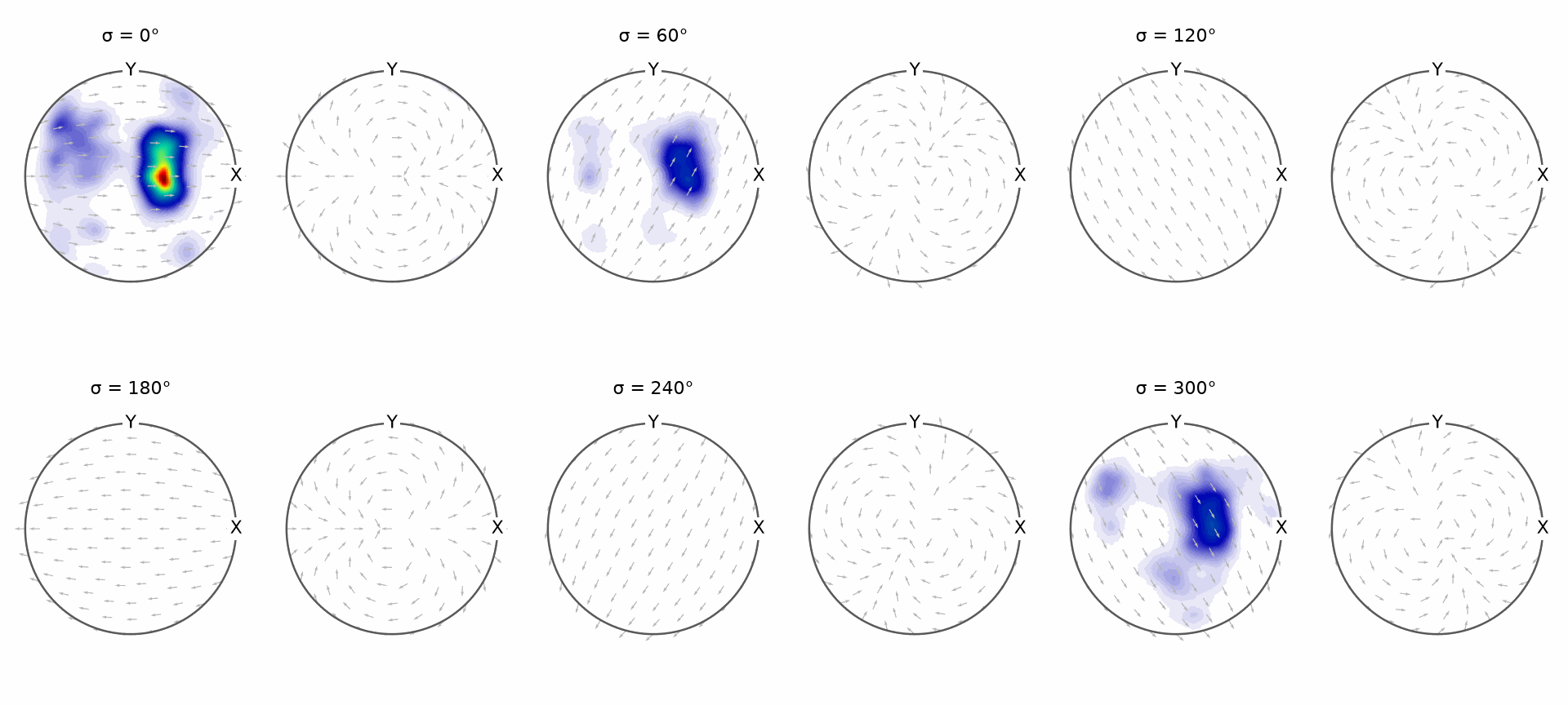
The peaks follow the high-valued sample regions, while the background remains nonnegative. The printed minimum and mean check the two density constraints directly. The residual can be larger than for an unconstrained fit because those constraints remove otherwise admissible solutions. If the iteration limit was reached, the coefficients may not yet be optimal. Adjust maxIter or tol before making a quantitative comparison.

The key smoothing parameter is the kernel halfwidth. A larger halfwidth blends information over a wider angular neighbourhood. A very small halfwidth can overfit the samples.

psi = SO3DeLaValleePoussinKernel(halfwidth=2.5 * degree)
SO3FNarrow = interp(ori, S['values'], density=True, kernel=psi, resolution=5 * degree)
plot(SO3FNarrow, 'sigma')

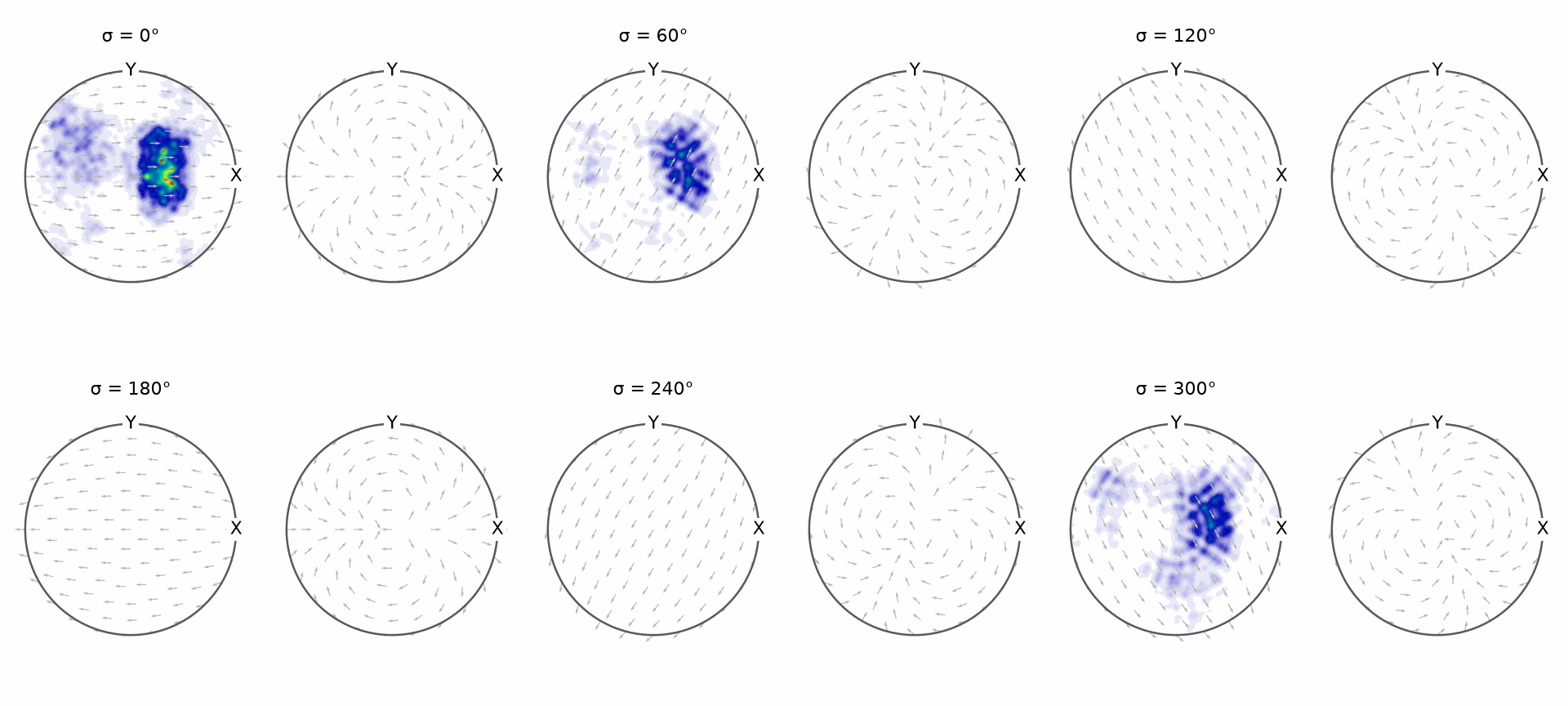
The centre spacing remains 5 degrees, so the change from the default fit comes from the 2.5 degree kernels. They produce narrower local features. Features that merely mirror the sample spacing are a warning that the halfwidth is too small. The RBF theory page develops this diagnostic and the other solver options.

Unconstrained RBF approximation

Omitting 'density' solves an unconstrained least-squares problem. As in the harmonic setting, the result may become negative and its mean need not equal 1.

SO3FRBF = interp(ori, S['values'])
relativeErrorRBF = norm(SO3FRBF.eval(ori) - S['values']) / norm(S['values'])
relativeErrorRBF

7.2691e-04

minimumRBFValue = min(SO3FRBF)[0]
minimumRBFValue

-6.0187

meanRBFValue = mean(SO3FRBF)
meanRBFValue

0.9800

plot(SO3FRBF, 'sigma')

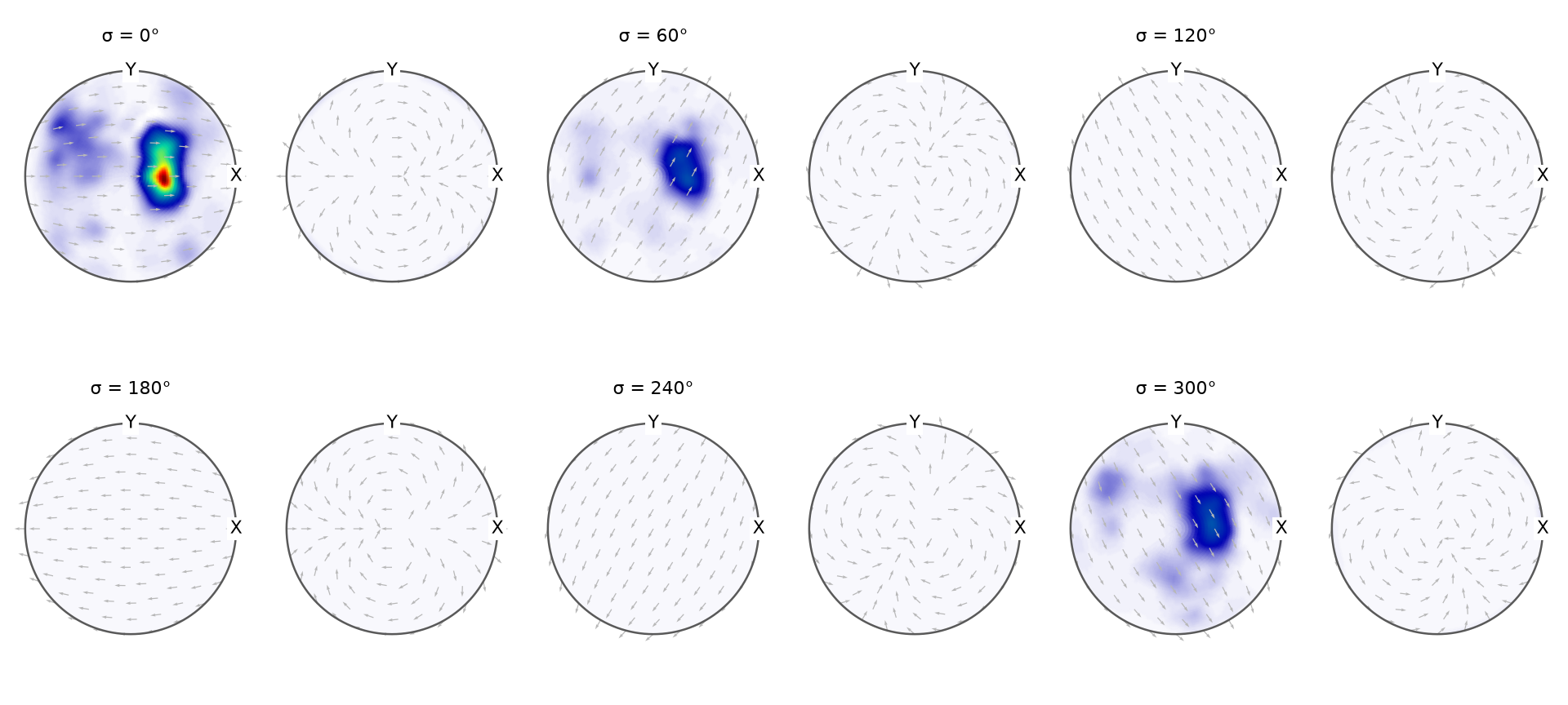
The unconstrained plot may follow the samples more closely, but the printed minimum and mean show why it should not automatically be interpreted as an ODF. Use this form for a general scalar response whose sign and mean are not prescribed. The same iteration-limit warning applies here: validate convergence before comparing residuals.

Fitting a Bingham distribution

SO3FunBingham.interpolate fits the samples with one Bingham distribution. The flag 'bingham' selects it through interp. The following controlled example begins with a fibre ODF and samples it on a coarse grid.

rng = np.random.default_rng(1)
cs = crystalFrame("1")
odf = fibreODF(fibre.rand(cs, rng=rng))
S3G = equispacedSO3Grid(cs, resolution=15 * degree)
v = odf.eval(S3G)

plot(odf)

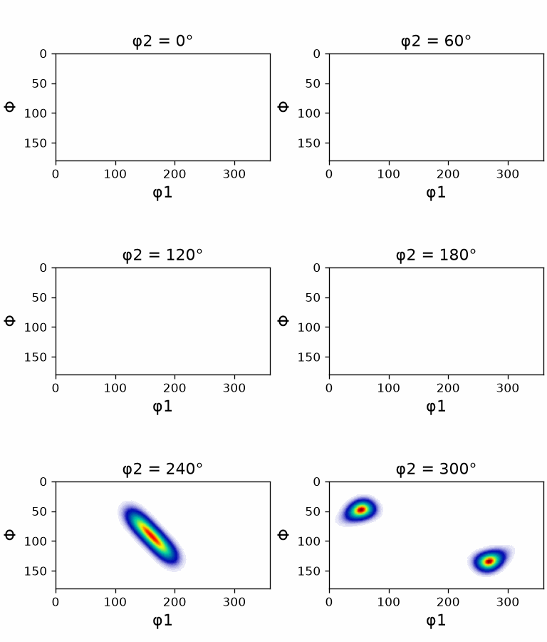
The source ODF has a continuous ridge of high values along one fibre. A Bingham distribution with two large equal concentrations and one zero is exactly that girdle shape, so a single component describes this ODF almost perfectly.

SO3FBingham = interp(S3G, v, 'bingham')
SO3FBingham

SO3FunBingham (1 → y↑→x)
  kappa : [92.064 92.063  0.517  0.   ]
  weight: 1

relativeErrorBingham = norm(SO3FBingham.eval(S3G) - v) / norm(v)
relativeErrorBingham

0.0045

plot(SO3FBingham)

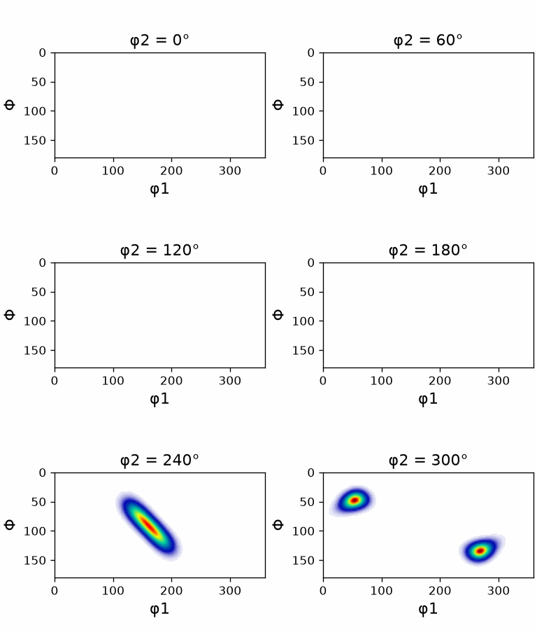
The printed concentrations show the girdle case, the residual is about one percent, and the two plots are hard to tell apart. One Bingham component has few parameters, so a source whose structure a girdle cannot hold - several separated components, say - is where this fit would fall short.

Bingham approximation currently works only for trivial symmetry. Do not use this route for the nontrivial symmetries: with a crystal symmetry the sample is first moved about its mean into one fundamental region, and the tensor of a density spread over that region is not the one of a Bingham distribution.

A response that is not an ODF

Density constraints are wrong for a property that may be negative or need not have mean 1. To make that distinction visible, consider noisy samples of

Here \(\omega(\mathbf{R})\) is the rotation angle, and \(\varphi_1(\mathbf{R})\) is the first Euler angle of \(\mathbf{R}\).

f = SO3FunHandle(lambda r: np.cos(r.angle()) * np.sin(3 * r.phi1) + 0.5)
plot(f, 'sigma')

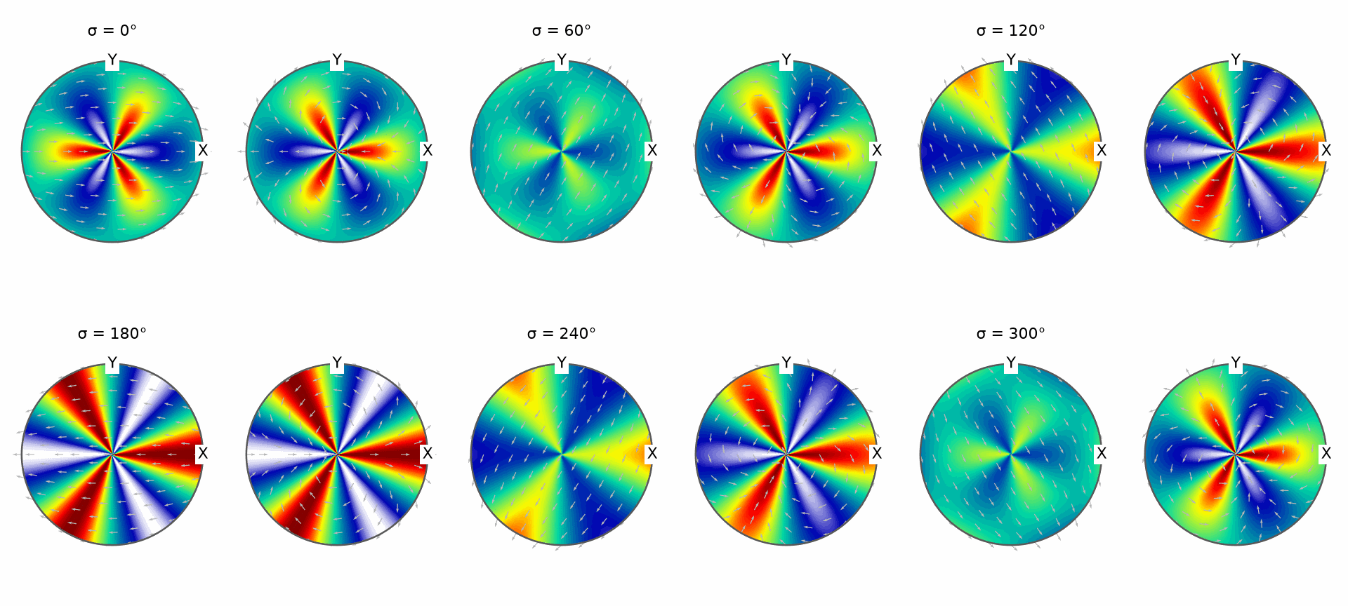
The exact response contains broad positive and negative lobes. A density fit would erase the negative part and change the intended quantity.

ori2 = orientation.rand(100000, rng=rng)
val2 = f.eval(ori2)
val2 = val2 + rng.standard_normal(val2.shape) * 0.05 * np.std(val2, ddof=1)

Fit the same 100,000 noisy samples with an unconstrained harmonic model and an unconstrained RBF model. A 12 degree RBF centre grid keeps this teaching example practical while retaining the large set of observations.

FH = interp(ori2, val2, 'harmonic')
FH

SO3FunHarmonic (1 → y↑→x)
  bandwidth: 40
  mean     : 0.4999

plot(FH, 'sigma')

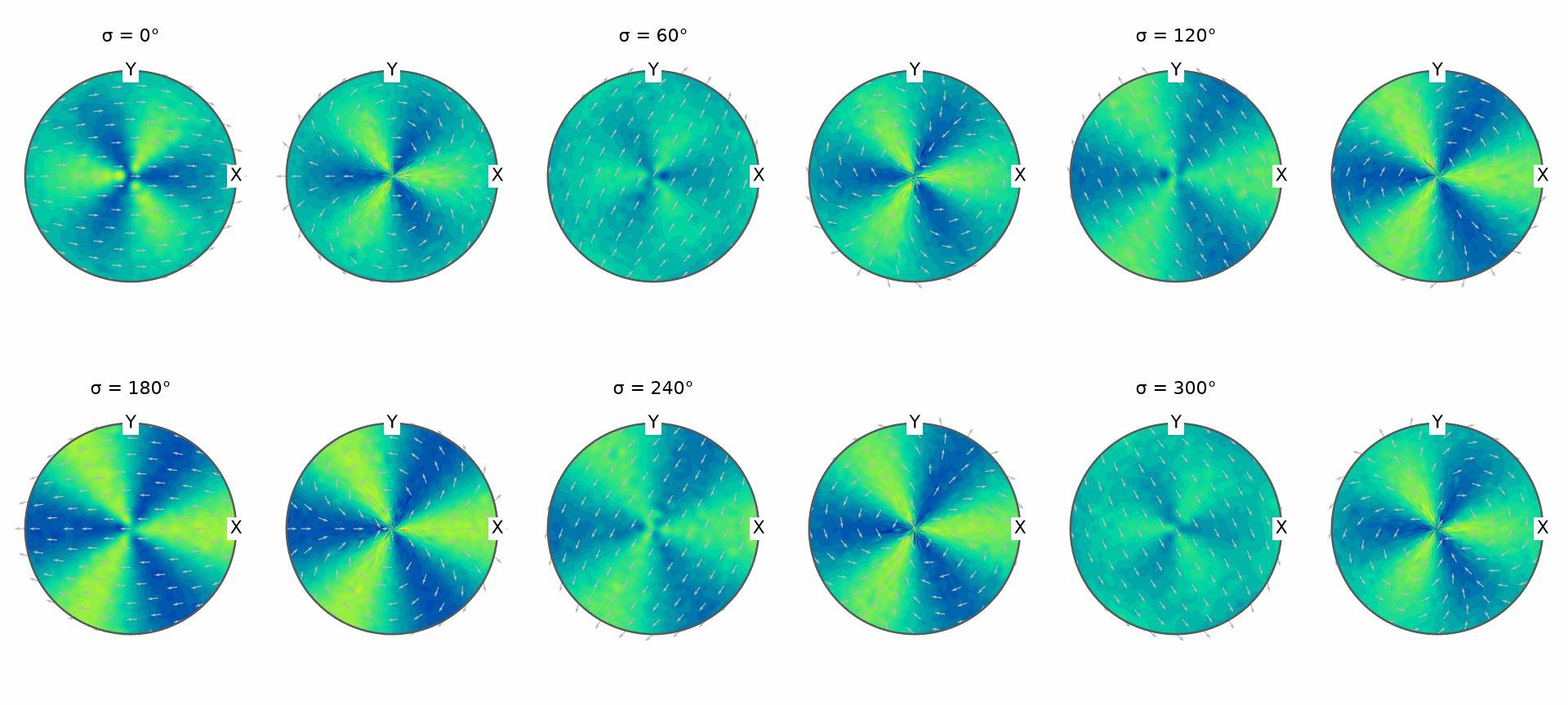
The harmonic fit recovers the broad alternating lobes, and it follows the samples more closely than the noise level warrants: its values run well outside the exact range of \(-0.5\) to \(1.5\), so the global series is fitting the noise along with the signal.

FK = interp(ori2, val2, resolution=12 * degree)
FK

SO3FunRBF (1 → y↑→x)
  multimodal components
    kernel: de la Vallee Poussin, halfwidth 12°
    center: 8520 orientations
    weight: 0.5
    Bunge Euler angles in degree
    phi1  Phi  phi2     weight
      90    6    90   -3.8e-05
      90    6   102  -0.000102
      90    6   114  -0.000317
      90    6   126  -7.35e-05
      90    6   138  -8.22e-05
       ⋮    ⋮     ⋮          ⋮
     330  174   150   1.75e-05
     330  174   162  -3.19e-05
     330  174   174   0.000319
     330  174   186  -6.71e-05
     330  174   198  -0.000131

plot(FK, 'sigma')

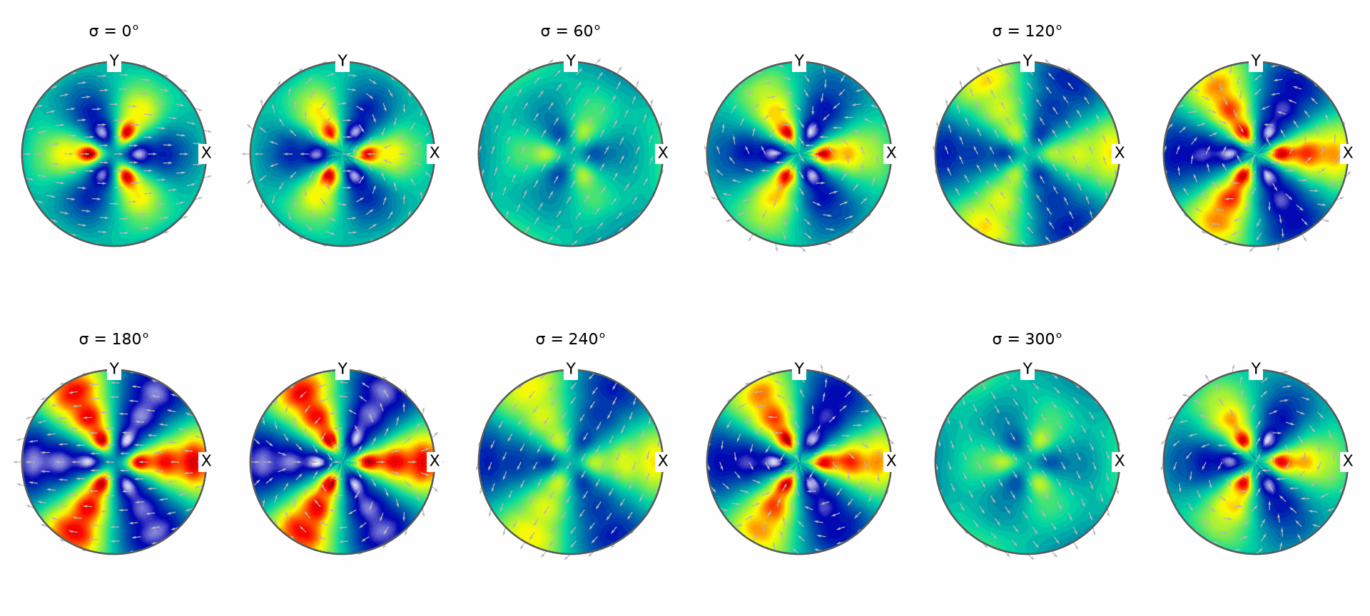
The RBF fit recovers the same sign changes through overlapping local kernels and stays much closer to the exact range. It reproduces the noisy samples less well and the underlying function better. Choose between the two by validation error on held-out samples and by computational cost, not by how closely each reproduces the data it was given.

References

• H. Schaeben, F. Bachmann, and J.-J. Fundenberger, Construction of weighted crystallographic orientations capturing a given orientation density function, Journal of Materials Science 52 (2017), 2077-2090, gives the constrained RBF formulation used for density approximation.
• C. Bingham, An antipodally symmetric distribution on the sphere, Annals of Statistics 2 (1974), 1201-1225, introduces the parametric distribution used by the Bingham fit.

Next

Continue with Harmonic Interpolation to tune bandwidth, regularisation, weights, and stopping criteria. Then use RBF-Kernel Interpolation to choose a kernel grid, halfwidth, density constraint, and least-squares solver.

Technical Details

min(f) returns the value with its position, so the minimum is min(f)[0]. The random fibre and the noise are drawn by NumPy.

@article{bachmann2010mtex,
  author  = {F. Bachmann and R. Hielscher and H. Schaeben},
  title   = {Texture Analysis with MTEX - Free and Open Source Software Toolbox},
  journal = {Solid State Phenomena},
  volume  = {160},
  pages   = {63-68},
  year    = {2010},
  doi     = {10.4028/www.scientific.net/SSP.160.63},
  url     = {https://doi.org/10.4028/www.scientific.net/SSP.160.63}
}