RBF-Kernel Approximation from Discrete Data

Approximating Orientation-Dependent Functions from Discrete Data defines the shared approximation problem and compares harmonic, RBF, and Bingham models. This page assumes that an RBF model is appropriate and shows how to choose density constraints, kernel halfwidth, centre orientations, and a least-squares solver.

RBF approximation is often useful for an ODF or another density when the number of observations and their noise level are not too large. It can also fit a general scalar response, but only 'density' imposes the nonnegativity and mean-1 constraints required of a density.

import time

import matplotlib.pyplot as plt
import numpy as np

from mtex import *

plottingConvention.default('y↑→x')

A noisy density data set

Start with the data used on the preceding two pages. This time the noise standard deviation is 20 percent of the standard deviation of the supplied values.

rng = np.random.default_rng(1)
fname = mtexdatafile('dubnaValues')
ori, S = loadOrientation(fname, columnNames=['phi1', 'Phi', 'phi2', 'values'])
val = S['values'] + rng.standard_normal(S['values'].shape) * 0.2 * np.std(S['values'], ddof=1)

plotSection(ori, val, 'sigma', all=True)

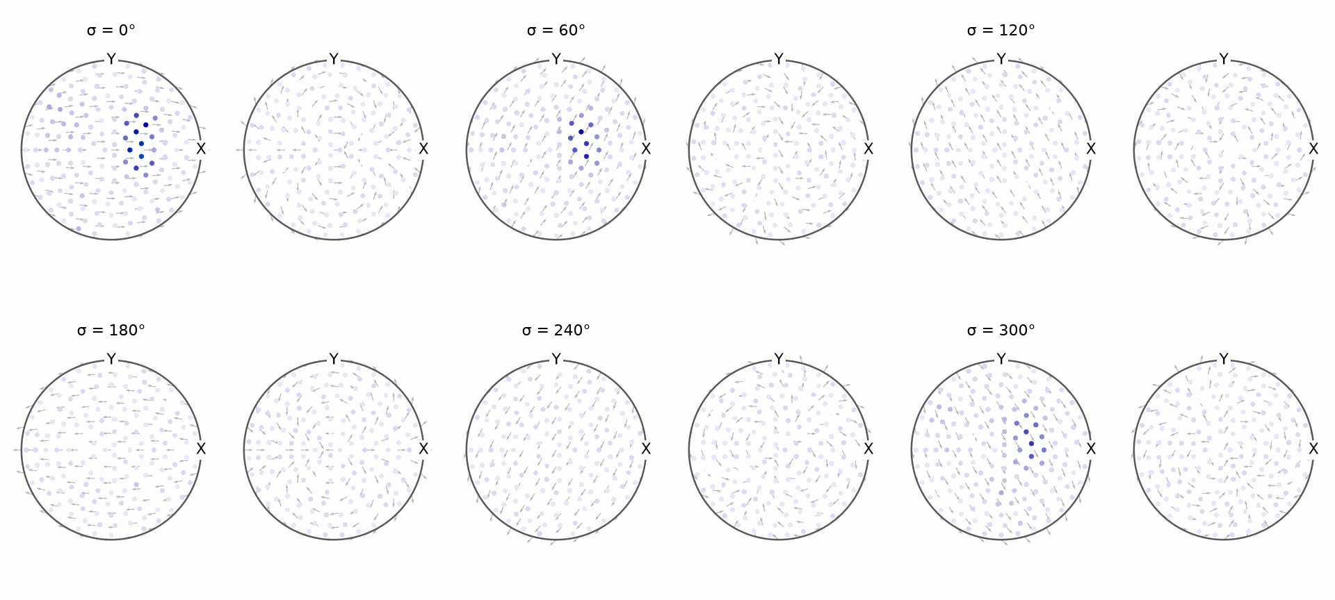
The broad high-value regions remain visible, but individual markers vary much more than on the harmonic page. The noise-free values S['values'] are retained only so that this controlled example can later measure recovery error. They would not be available for an unknown experimental response.

Fit a density

interp uses an RBF model by default and calls SO3FunRBF.interpolate. The 'density' flag selects modified least squares, 'mlsq'. This solver constrains the kernel weights to be nonnegative, and MTEX normalizes the fitted function to mean 1.

SO3FDensity = interp(ori, val, density=True)
SO3FDensity

SO3FunRBF (1 → y↑→x)
  multimodal components
    kernel: de la Vallee Poussin, halfwidth 5°
    center: 73610 orientations
    weight: 1
    Bunge Euler angles in degree
    phi1  Phi  phi2    weight
      90  2.5    90  2.03e-07
      90  2.5    95  3.98e-07
      90  2.5   100  9.05e-07
      90  2.5   105  6.66e-07
      90  2.5   110  8.11e-07
       ⋮    ⋮     ⋮         ⋮
      30  178   125   2.5e-08
      30  178   130  2.48e-07
      30  178   135  1.76e-07
      30  178   140  1.96e-07
      30  178   145  5.11e-07

minimumDensityValue = min(SO3FDensity)[0]
minimumDensityValue

0.0027

meanDensityValue = mean(SO3FDensity)
meanDensityValue

1

relativeDataResidual = norm(SO3FDensity.eval(ori) - val) / norm(val)
relativeDataResidual

0.1620

plot(SO3FDensity, 'sigma')
mtexColorbar()

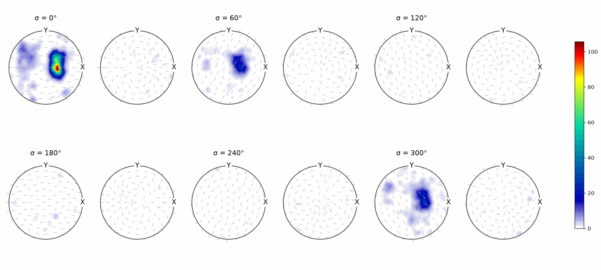
The fit retains the broad peaks while smoothing the marker-to-marker fluctuations. Its printed minimum and mean verify the density constraints. A nonzero residual is expected because a smooth constrained model cannot reproduce every noisy value. If the fit reaches the 100-iteration 'mlsq' limit, its coefficients may not yet be optimal.

Fit without density constraints

Omitting 'density' selects unconstrained LSQR. The kernel grid still smooths the data, so the result is not literally “undenoised.” It simply has more freedom to reduce the sample residual, including by using negative weights or changing the mean.

SO3FFree = interp(ori, val)
SO3FFree

SO3FunRBF (1 → y↑→x)
  multimodal components
    kernel: de la Vallee Poussin, halfwidth 5°
    center: 119088 orientations
    weight: 0.9613
    Bunge Euler angles in degree
    phi1  Phi  phi2     weight
      90  2.5    90   2.16e-05
      90  2.5    95   1.08e-05
      90  2.5   100  -3.34e-06
      90  2.5   105  -1.03e-06
      90  2.5   110   1.24e-05
       ⋮    ⋮     ⋮          ⋮
      30  178   125  -9.61e-07
      30  178   130   9.85e-06
      30  178   135    8.8e-06
      30  178   140   9.21e-06
      30  178   145   1.15e-05

minimumFreeValue = min(SO3FFree)[0]
minimumFreeValue

-7.2995

meanFreeValue = mean(SO3FFree)
meanFreeValue

0.9613

relativeFreeResidual = norm(SO3FFree.eval(ori) - val) / norm(val)
relativeFreeResidual

6.5598e-04

plot(SO3FFree, 'sigma')
mtexColorbar()

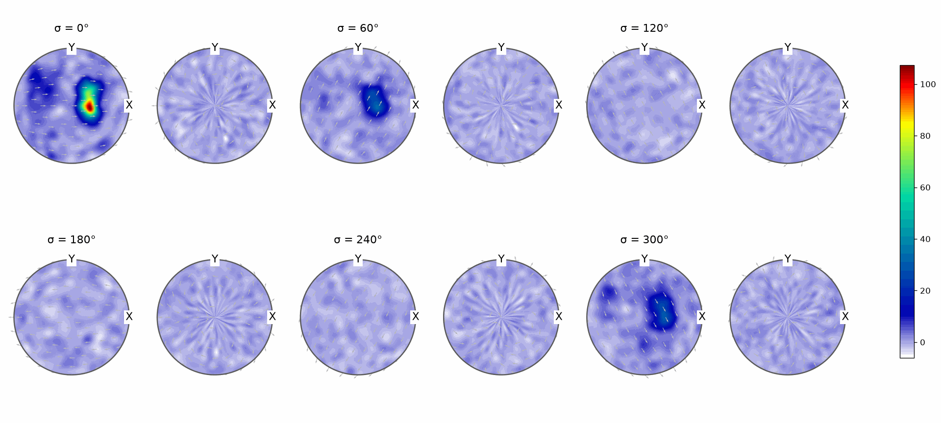
The unconstrained residual is smaller, but the printed minimum and mean show that this fit is not automatically a density. Fine-scale features that only reduce the training residual are possible overfitting, not evidence that the unconstrained model is physically better.

Separate halfwidth from centre spacing

The kernel halfwidth controls how far each centre influences neighbouring orientations. A large halfwidth produces a smooth fit. A halfwidth that is small relative to the data spacing can reproduce noise.

By default, the halfwidth option also sets the resolution of the equispaced centre grid. That coupling changes both the kernel shape and the number of unknown weights. Specify resolution separately when the aim is to isolate the effect of halfwidth.

SO3FNarrow = interp(ori, val, density=True, halfwidth=2 * degree, resolution=5 * degree)
SO3FNarrow

SO3FunRBF (1 → y↑→x)
  multimodal components
    kernel: de la Vallee Poussin, halfwidth 2°
    center: 119086 orientations
    weight: 1
    Bunge Euler angles in degree
    phi1  Phi  phi2    weight
      90  2.5    90  4.69e-06
      90  2.5    95  2.97e-08
      90  2.5   100   2.8e-06
      90  2.5   105  1.47e-07
      90  2.5   110  1.82e-06
       ⋮    ⋮     ⋮         ⋮
      30  178   125  3.15e-06
      30  178   130   2.5e-06
      30  178   135  1.66e-06
      30  178   140  1.31e-06
      30  178   145  2.97e-06

plot(SO3FNarrow, 'sigma')

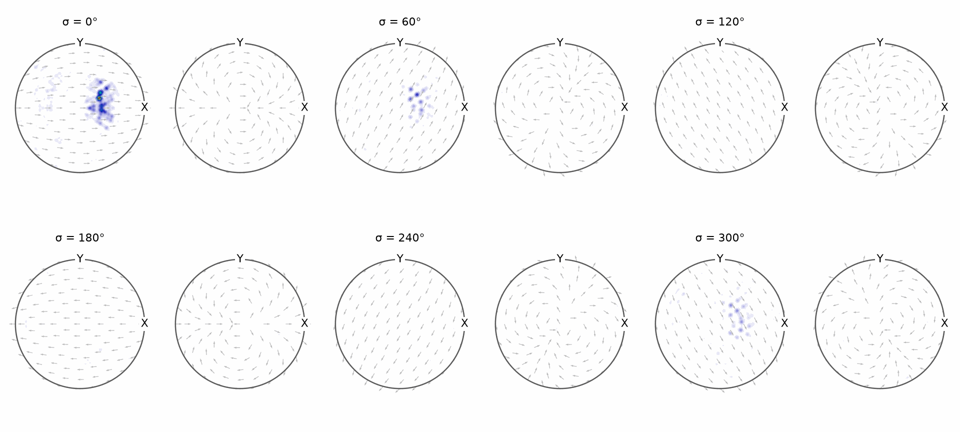
The 2 degree kernels are narrower than the fixed 5 degree centre spacing. The resulting small-scale peaks track local samples rather than the broad structure. As a rule of thumb, start with a halfwidth at least as large as the resolution of the data, then validate that choice.

SO3FSmooth = interp(ori, val, density=True, halfwidth=10 * degree, resolution=5 * degree)
SO3FSmooth

SO3FunRBF (1 → y↑→x)
  multimodal components
    kernel: de la Vallee Poussin, halfwidth 10°
    center: 69896 orientations
    weight: 1
    Bunge Euler angles in degree
    phi1  Phi  phi2    weight
      90  2.5    95  4.73e-08
      90  2.5   100  1.95e-07
      90  2.5   105  2.21e-07
      90  2.5   110   1.3e-07
      90  2.5   115  4.99e-08
       ⋮    ⋮     ⋮         ⋮
      30  178   125  1.51e-08
      30  178   130  1.42e-08
      30  178   135  1.19e-08
      30  178   140  2.15e-08
      30  178   145  5.17e-08

plot(SO3FSmooth, 'sigma')

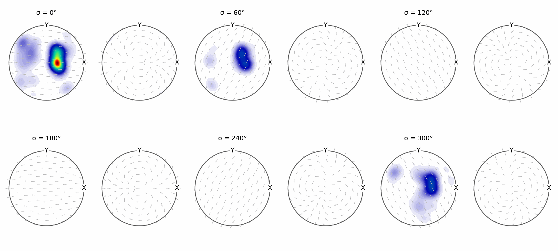
The 10 degree kernels overlap much more. The broad peaks remain while narrow fluctuations merge into a smoother surface.

Supply the centre orientations

Use SO3Grid when the centre grid must be controlled directly. Its symmetry should match the sample orientations.

S3G = equispacedSO3Grid(ori.CS, resolution=5 * degree)
S3G

SO3Grid (1 → y↑→x)
  size      : 119088
  resolution: 5°

SO3FGrid = interp(ori, val, density=True, SO3Grid=S3G)
SO3FGrid

SO3FunRBF (1 → y↑→x)
  multimodal components
    kernel: de la Vallee Poussin, halfwidth 5°
    center: 73610 orientations
    weight: 1
    Bunge Euler angles in degree
    phi1  Phi  phi2    weight
      90  2.5    90  2.03e-07
      90  2.5    95  3.98e-07
      90  2.5   100  9.05e-07
      90  2.5   105  6.66e-07
      90  2.5   110  8.11e-07
       ⋮    ⋮     ⋮         ⋮
      30  178   125   2.5e-08
      30  178   130  2.48e-07
      30  178   135  1.76e-07
      30  178   140  1.96e-07
      30  178   145  5.11e-07

plot(SO3FGrid, 'sigma')

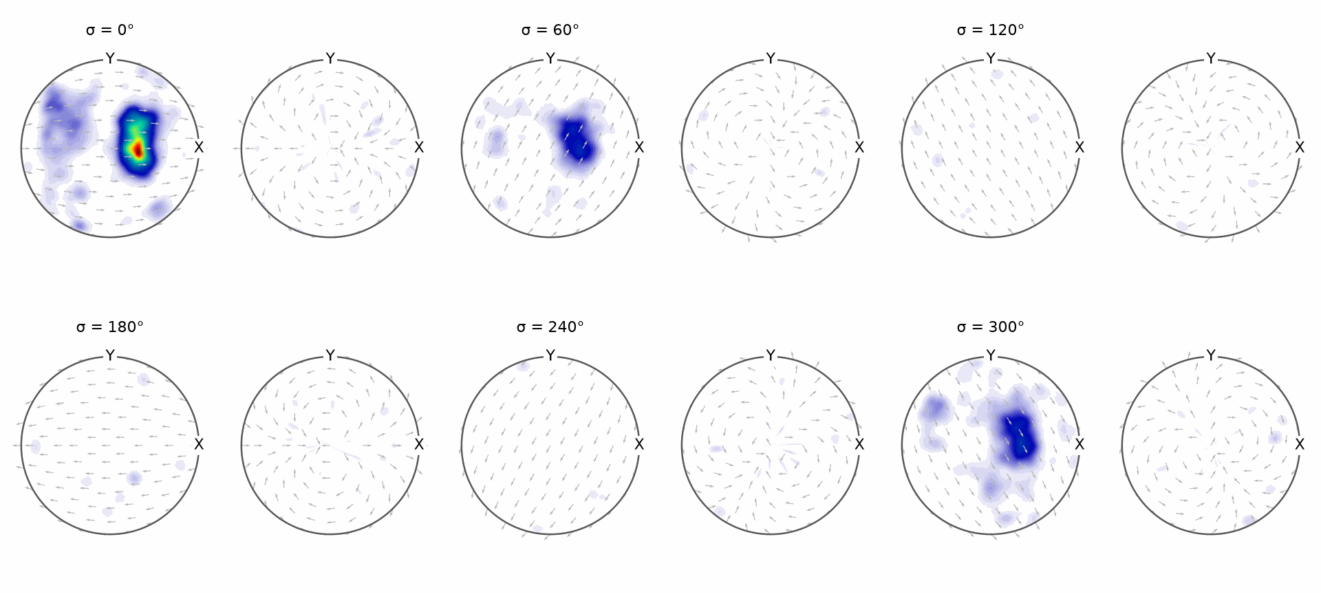
The fitted function reports the supplied 5 degree centre grid. The plot resembles the default density fit because that fit makes the same grid choice; the explicit form is useful when several fits must share centres.

Measure a halfwidth sweep

Keep the centre resolution at 5 degrees while changing only halfwidth. The error is measured against the noise-free values in this simulation, not against the noisy training values.

hw = np.array([20, 15, 12.5, 10, 7.5, 5, 2.5])
err = np.zeros(len(hw))
for k in range(len(hw)):
  SO3Fhw = interp(ori, val, density=True, halfwidth=hw[k] * degree, resolution=5 * degree)
  err[k] = norm(SO3Fhw.eval(ori) - S['values']) / norm(S['values'])

plt.figure(figsize=(6, 3.5))
plt.plot(hw, err, 'o--')
plt.gca().invert_xaxis()
plt.xlabel('halfwidth [deg]')
plt.ylabel('relative recovery error')

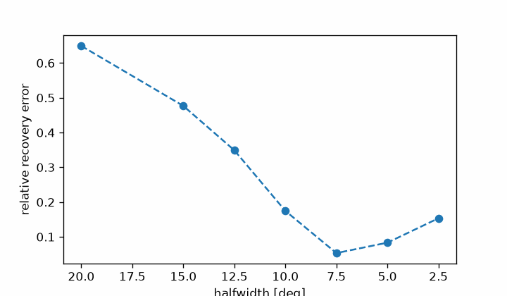
Read the curve from broad kernels on the left towards narrow kernels on the right. The minimum balances smoothing bias against sensitivity to noise. A sweep that also changed the centre-grid resolution would mix two effects; this one changes the kernel alone. If the fits reach the iteration cap, the result is the best of the capped fits rather than a claim that every solver reached its optimum.

bestIndex = int(np.argmin(err))
bestHalfwidth = hw[bestIndex]
bestHalfwidth

7.5000

bestRecoveryError = err[bestIndex]
bestRecoveryError

0.0533

SO3FBest = interp(ori, val, density=True, halfwidth=bestHalfwidth * degree, resolution=5 * degree)
plot(SO3FBest, 'sigma')

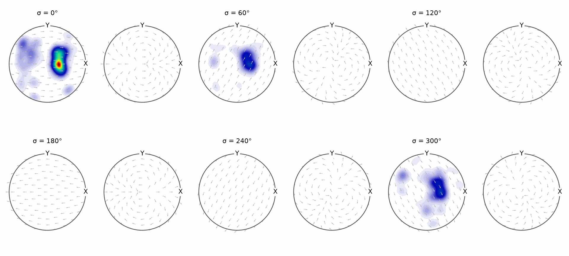
The selected fit retains the broad regions while suppressing much of the added noise. A small training residual alone could not select it; the known noise-free target makes this a validation experiment. With real data, use held-out samples or independent physical knowledge instead.

If too few observations constrain too many centre weights, the system is underdetermined. A small halfwidth does not supply the missing information; use fewer centres, a stronger constraint, or additional smoothness assumptions.

Choose another kernel

halfwidth constructs a SO3DeLaValleePoussinKernel. Pass kernel to use another rotational kernel function.

psi = SO3AbelPoissonKernel(halfwidth=5 * degree)
psi

SO3AbelPoissonKernel
  bandwidth: 48
  halfwidth: 5°

SO3FAbel = interp(ori, val, density=True, kernel=psi, resolution=5 * degree)
plot(SO3FAbel, 'sigma')

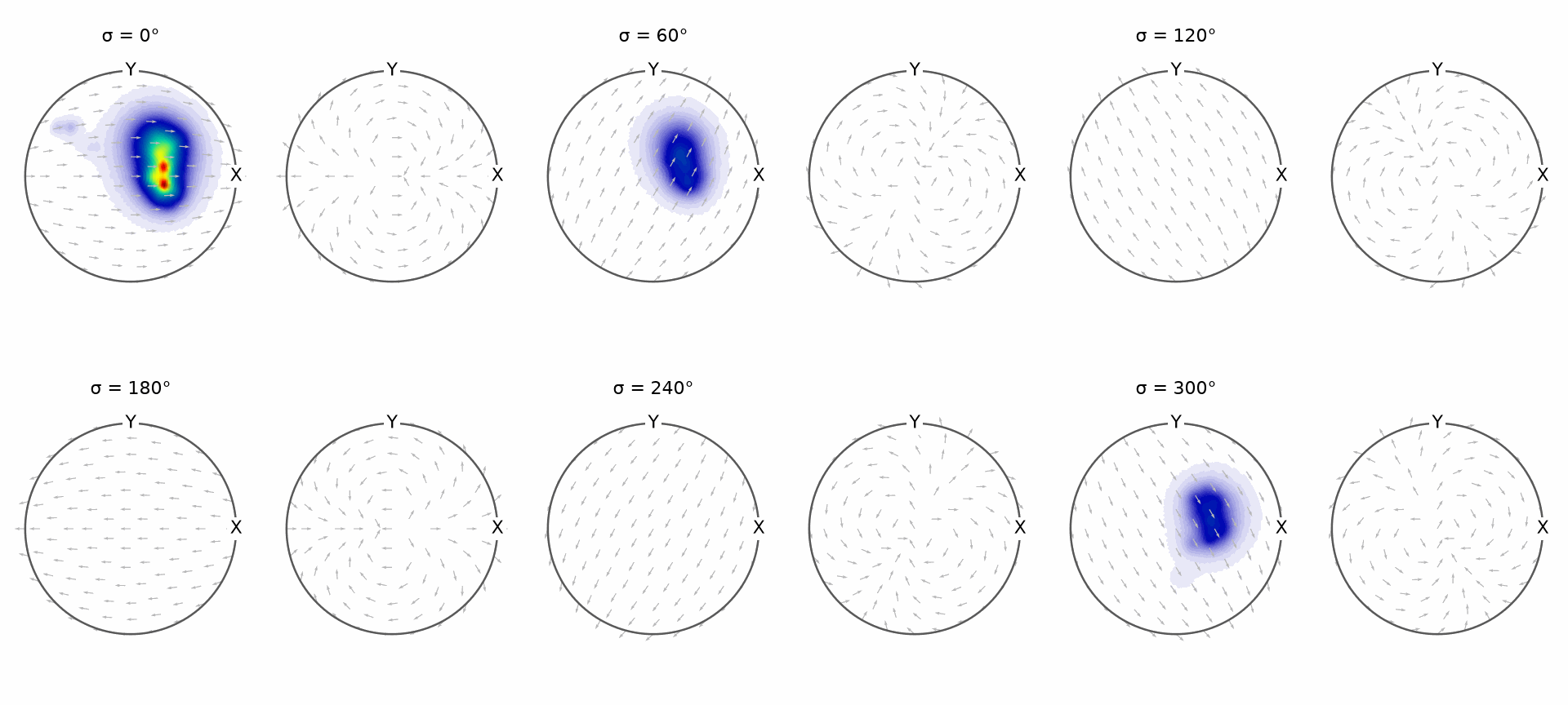
The Abel-Poisson fit places its peaks in the same broad regions, but its tails and peak shapes differ from the de la Vallee Poussin result. Kernel family and halfwidth are separate modelling choices.

Exact interpolation

If the values are noise-free, the input orientations themselves can be used as kernel centres with exact=True. For distinct nodes and a positive-definite kernel, the resulting kernel matrix is symmetric and positive definite, so the linear system has a unique exact solution.

That matrix is generally dense. Construction, solution, and later evaluation can therefore become prohibitively expensive for the complete data set. The example uses a reproducible subset to make the cost visible without attempting the original all-node dense system.

exactNodes = ori[::20]
exactValues = S['values'][::20]
numberOfExactNodes = exactNodes.size
numberOfExactNodes

522

t = time.perf_counter()
SO3FExact = SO3FunRBF.interpolate(exactNodes, exactValues, exact=True, halfwidth=7.5 * degree)
exactFitTime = time.perf_counter() - t

plot(SO3FExact, 'sigma')

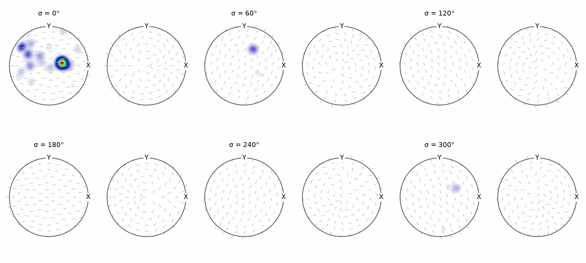
The exact-centre fit follows the noise-free subset closely. Every value moves the weight of the kernel at its own node, so noise in the values would go straight into the fit, which is why exact interpolation is unsuitable for noisy data. Because these centres are not a structured grid, later evaluations are slower than for a grid-centred RBF model.

The iterative solver stops at a requested tolerance or iteration limit, so its computed residual need not reach machine precision. Exact centres make an exact solution available; they do not force the iterative solver to reach it.

relativeExactResidual = norm(SO3FExact.eval(exactNodes) - exactValues) / norm(exactValues)
relativeExactResidual

0.0144

minimumExactValue = min(SO3FExact)[0]
minimumExactValue

0.0023

The printed residual checks how closely this run solved the system. Exact interpolation of nonnegative values takes the positive solver here as well, so the minimum stays positive; with values of both signs the fit is unconstrained and may become negative.

Choose a least-squares solver

The harmonic page introduces LSQR stopping conditions. RBF interpolation uses tol and maxIter in the same spirit, but its defaults depend on the solver: unconstrained 'lsqr' uses at most 30 iterations, whereas density-constrained 'mlsq' uses at most 100. Both default to tol=1e-3.

The two solvers serve different constraints:

• 'lsqr' is the fast default for an unconstrained least-squares fit.
• 'mlsq' enforces positive normalized weights and is selected by 'density', or by values of one sign at fewer than 10,000 nodes.

With withIterations=True, SO3FunRBF.interpolate also returns the iteration count, not a convergence flag. Compare residuals and fits when the count reaches the selected limit.

f1, iter1 = SO3FunRBF.interpolate(ori, val, withIterations=True)
residualNorm1 = norm(f1.eval(ori) - val)
print(f'default: iterations {iter1}, residual norm {residualNorm1:.6g}')

f2, iter2 = SO3FunRBF.interpolate(ori, val, tol=1e-15, maxIter=100, withIterations=True)
residualNorm2 = norm(f2.eval(ori) - val)
print(f'tight tol: iterations {iter2}, residual norm {residualNorm2:.6g}')

default: iterations 8, residual norm 0.589965
tight tol: iterations 41, residual norm 0.374288

If the second run reaches 100 iterations, it has stopped at maxIter rather than satisfying the very small tolerance. Increase the limit only when the additional accuracy matters to validation or interpretation.

The maths behind RBF approximation

An RBF model places one rotational kernel \(\Psi\) at each centre \(R_n\):

Here \(\omega(x,R_n)\) is the rotation angle between the evaluation orientation and the centre. The coefficients \(c_n\) are the unknown weights. With sample pairs \((x_m,v_m)\), unconstrained fitting solves

The kernel matrix is sparse in the usual grid-centred approximation because MTEX neglects interactions outside a halfwidth-dependent angular neighbourhood. The exact flag evaluates every interaction, which is why that matrix loses the computational advantage.

For a density fit, modified least squares additionally requires nonnegative coefficients with a prescribed sum. MTEX then normalizes the resulting RBF function to mean 1. These constraints explain why a density fit can have a larger sample residual than unconstrained LSQR.

References

• H. Schaeben, F. Bachmann, and J.-J. Fundenberger, Construction of weighted crystallographic orientations capturing a given orientation density function, Journal of Materials Science 52 (2017), 2077-2090, develops the positive normalized RBF approximation implemented by 'mlsq'.

Next

Continue with Approximation and Quadrature to replace scattered observations by values on a quadrature grid and compute a harmonic representation of a known orientation-dependent function.

Technical Details

MATLAB’s second output of SO3FunRBF.interpolate is withIterations=True here. MATLAB also offers the solvers 'mlrl', 'lsqnonneg', 'lsqlin' and 'nnls'; the port has 'lsqr' and 'mlsq'. The noise is drawn by NumPy. MATLAB evaluates a sum of kernels through the sparse matrix of the kernel at every point; the port evaluates one of more than two million kernel terms through its harmonic form at the bandwidth of the kernel, which reproduces the sum to about \(4\mathbin{\cdot}10^{-4}\). The residuals at the samples cannot fall below that: the tight LSQR run converges in 41 iterations as MATLAB’s does, which reports a residual norm of \(7.9\mathbin{\cdot}10^{-13}\), while the port’s evaluation gives 0.37. MATLAB’s density fits keep 71802, 119075 and 69937 centres where the port’s keep 73610, 119086 and 69896.

@article{bachmann2010mtex,
  author  = {F. Bachmann and R. Hielscher and H. Schaeben},
  title   = {Texture Analysis with MTEX - Free and Open Source Software Toolbox},
  journal = {Solid State Phenomena},
  volume  = {160},
  pages   = {63-68},
  year    = {2010},
  doi     = {10.4028/www.scientific.net/SSP.160.63},
  url     = {https://doi.org/10.4028/www.scientific.net/SSP.160.63}
}