Grain Boundary Properties

A grain boundary is stored as short segments between neighbouring EBSD measurements that belong to different grains. Most properties come in pairs: two pixels, grains, phases, and the misorientation between them. The remaining properties describe the segment’s geometry and its place in the boundary network.

This page assumes that the map has already been divided into grains as in Grain Reconstruction. Select Grain Boundaries covers phase and grain selection. Grain Boundaries explains the physical meaning of a boundary trace in a two-dimensional section.

import numpy as np
from mtex import *

# load the example map in its specimen plotting frame
plottingConvention.default('y↑→x')
ebsd = mtexdata('twins')
for name in ('error', 'bands'):
  del ebsd.prop[name]

# reconstruct the grains
grains = calcGrains(ebsd, angle=10 * degree, minPixel=3)

Preserve the segment-to-pixel relation

This page uses ebsdId to inspect the pixel pair beside each segment. Boundary simplification and refinement change the segment count, and a resampled segment no longer lies between one specific pixel pair. The smoothBoundary options simplify=False and refine=False preserve that relation while smoothing.

grains = grains.smoothBoundary(5, simplify=False, refine=False)

# draw the grains and overlay the complete boundary network
plot(grains, faceColor=[0.9, 0.9, 0.9], micronbar='off')
gB = grains.boundary
hold(True)
plot(gB, lineWidth=2)
hold(False)

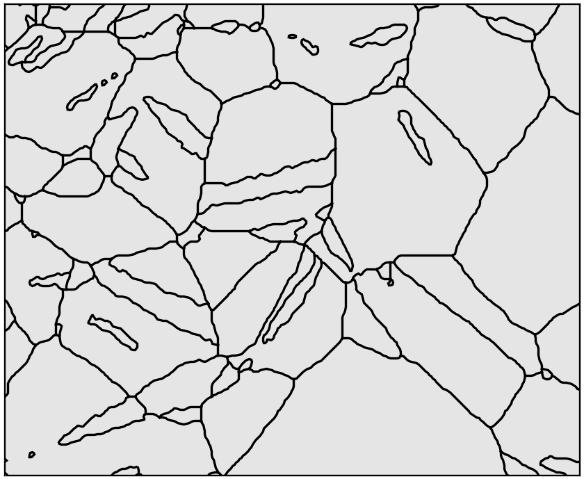
The thick black lines show that the boundary is a network of individual segments. Each segment separates one pair of neighbouring measurements.

The two sides of a segment

ebsdId, grainId, and phaseId are \(N \times 2\) matrices. Each row records what lies on the two sides of one segment. Consider the boundary of one small grain:

gB4 = grains['id', 9].boundary
gB4

grainBoundary (y↑→x)
  size: 8 segments, 1 chains
  segments  length  mineral 1  mineral 2
         8  1.3 µm  Magnesium  Magnesium

The object summary reports eight segments. Its ebsdId property is therefore an 8 by 2 matrix.

gB4.ebsdId

array([[ 841,  842],
       [1008, 1009],
       [1176, 1009],
       [1177, 1010],
       [1011, 1010],
       [ 843, 1010],
       [ 843,  842],
       [ 675,  842]], dtype=int32)

These values are measurement IDs, not positions in the current list. IDs and list positions differ as soon as measurements have been removed from the map. Indexing by ID must say so explicitly.

ebsd['id', gB4.ebsdId]

EBSD (y↑→x)
  size: 8 × 2 grid
  Phase  Orientations  Mineral    Color         Symmetry  Crystal reference frame
  1      16 (100%)     Magnesium  LightSkyBlue  6/mmm     Magnesium
    Id  Phase            orientation   bc   bs  grainId  mad
   841      1    (4.9°,80.4°,195.2°)  167  170        1  0.5
   842      1  (115.3°,15.6°,218.2°)  170  176        9  0.7
  1008      1    (4.6°,80.7°,195.4°)  156  160        1  0.4
  1009      1  (113.7°,15.5°,219.3°)  164  158        9  0.5
  1176      1    (4.5°,80.7°,195.2°)  168  171        1  0.3
  1009      1  (113.7°,15.5°,219.3°)  164  158        9  0.5
  1177      1    (4.7°,80.8°,195.4°)  174  181        1  0.5
  1010      1  (114.7°,15.7°,218.5°)  182  174        9  0.5
  1011      1    (4.4°,80.5°,195.2°)  176  168        1  0.4
  1010      1  (114.7°,15.7°,218.5°)  182  174        9  0.5
   843      1    (4.4°,80.5°,195.1°)  174  197        1  0.3
  1010      1  (114.7°,15.7°,218.5°)  182  174        9  0.5
   843      1    (4.4°,80.5°,195.1°)  174  197        1  0.3
   842      1  (115.3°,15.6°,218.2°)  170  176        9  0.7
   675      1    (4.9°,80.4°,195.2°)  176  196        1  0.5
   842      1  (115.3°,15.6°,218.2°)  170  176        9  0.7
  scan unit     : um
  X × Y         : [1.8 → 2.7] × [1.2 → 2.1]
  square lattice: spacing 0.3

The grain IDs on the two sides reveal the local grain arrangement.

gB4.grainId

array([[1, 9],
       [1, 9],
       [1, 9],
       [1, 9],
       [1, 9],
       [1, 9],
       [1, 9],
       [1, 9]], dtype=int32)

Grain 9 has grain 1 on the far side of all eight segments. Grain 9 is therefore an inclusion: it is entirely surrounded by one other grain.

plot(grains['id', 9], faceColor='DarkBlue', micronbar='off')
hold(True)
plot(grains['id', 1], faceColor='LightCoral')
hold(False)

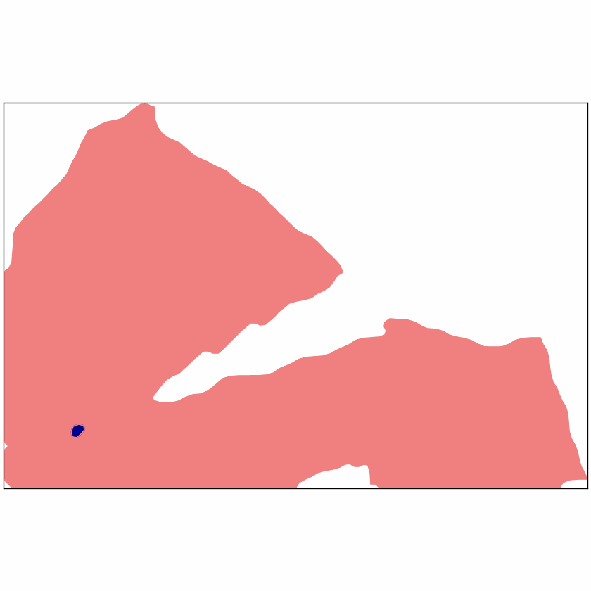
The dark-blue inclusion sits wholly inside the coral grain. The plot is the spatial counterpart of the repeated pair [1 9] above.

From segments to chains

A chain is a maximal run of segments laid end to end. It runs from one junction to the next and never passes through a junction. Every segment belongs to exactly one chain. The same two grains lie on its two sides along the entire chain.

A junction is a vertex where the number of meeting segments is not two. It need not be a triple point. For example, the end of a boundary at the map rim is a junction but not a point where three real grains meet.

The inclusion boundary reaches no junction and closes onto itself. Its eight segments consequently form one closed chain.

print(f'{"chainId":>10s}{"chainSize":>12s}{"isClosed":>11s}')
print(f'{gB4.chainId[0]:>10d}{gB4.chainSize[0]:>12d}{str(bool(gB4.isClosed[0])):>11s}')

   chainId   chainSize   isClosed
         0           8       True

arcLength is the cumulative length from the start of a chain to the end of each segment. chainLength repeats the total length on every segment, so either property remains aligned with the boundary list during indexing.

The misorientation across a segment

A segment’s misorientation is the rotation from the orientation of its second pixel to that of its first. It follows the column order of ebsdId and can be reproduced from the two pixel orientations.

gB4[0].misorientation

misorientation (Magnesium → Magnesium)
  antipodal: true
  Bunge Euler angles in degree
  phi1   Phi  phi2
  29.6  86.1   210

inv(ebsd['id', gB4.ebsdId[0, 1]].orientations) * ebsd['id', gB4.ebsdId[0, 0]].orientations

misorientation (Magnesium → Magnesium)
  Bunge Euler angles in degree
  phi1   Phi  phi2
  29.6  86.1   210

The two rotations agree, but only the stored one has its antipodal flag set. A boundary has no preferred side, so MTEX treats that rotation and its inverse as the same boundary misorientation. The rotation computed directly from two ordered orientations retains its direction.

A list of misorientations is meaningful only when every segment relates the same two phases. Select the phase pair before analysing angles or axes.

gB_Mg = gB['Magnesium', 'Magnesium']

# plot the misorientation angle on each magnesium boundary segment
moriAngle = gB_Mg.misorientation.angle() / degree
plot(gB_Mg, moriAngle, lineWidth=4, micronbar='off')
mtexColorbar(title='misorientation angle (°)')

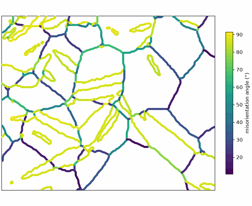
Long runs share nearly the same colour, as expected for segments along one twin boundary. Most non-twin boundaries form the contrasting shorter runs.

The dominant magnesium twin has a misorientation angle of 86.3 degrees. In this map, 52.8 percent of the magnesium segments are within 3 degrees of that angle, and the median angle is 84.3 degrees.

fractionNearTwin = np.mean(np.abs(moriAngle - 86.3) < 3)
medianMoriAngle = np.median(moriAngle)
print(f'fraction near the twin angle {fractionNearTwin:.4f}, median angle {medianMoriAngle:.4f}')

fraction near the twin angle 0.5282, median angle 84.2556

The high fraction confirms that this specimen is dominated by twin boundaries. Twinning develops that selection.

Which way a segment runs

direction is the direction of the segment trace. Its angle to the misorientation axis is used when classifying tilt and twist boundaries. See Twist and Tilt. Compute the axis in specimen coordinates from the two pixel orientations. The stored misorientation alone no longer retains that specimen-frame information.

# compute misorientation axes in specimen coordinates
ori = ebsd['id', gB_Mg.ebsdId].orientations
axes = axis(ori[:, 0], ori[:, 1], antipodal=True)

# plot the angle between each axis and its raw segment direction
rawAxisTraceAngle = angle(gB_Mg.direction, axes) / degree
plot(gB_Mg, rawAxisTraceAngle, lineWidth=4, micronbar='off')
mtexColorbar(title='axis-to-trace angle (°)')

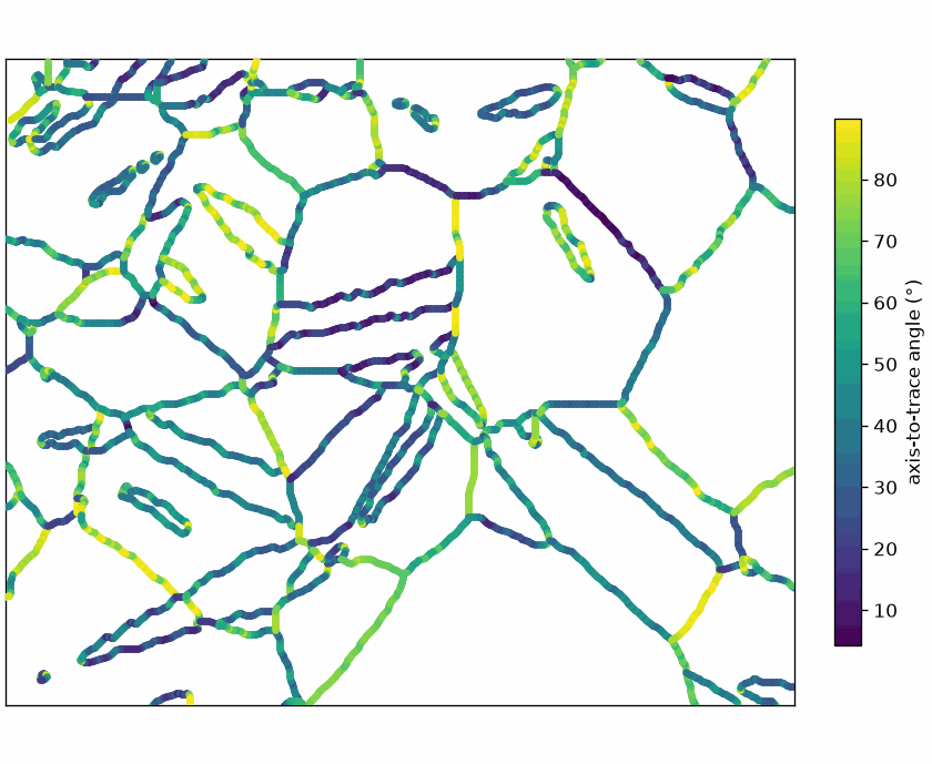
The colour flickers along boundaries that are straight on the scale of several pixels. This is the pixel staircase: one segment has only a few possible grid directions, regardless of the direction of the underlying boundary.

calcMeanDirection uses a window along each chain and never crosses a junction. An argument of 4 includes four neighbouring segments on each side of the segment.

meanDirection = gB_Mg.calcMeanDirection(4)
meanAxisTraceAngle = angle(meanDirection, axes) / degree
plot(gB_Mg, meanAxisTraceAngle, lineWidth=4, micronbar='off')
mtexColorbar(title='axis-to-mean-trace angle (°)')

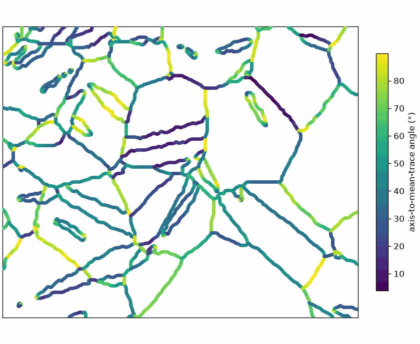
The flicker is suppressed, so nearby segments on one boundary now carry similar colours. The values differ from boundary to boundary, which is the information the flicker was hiding. The median angle is 43.2 degrees, and 10.5 percent of the segments lie below 20 degrees. The misorientation axes are therefore mostly not aligned with the traces in this section.

print(f'median axis-trace angle {np.median(meanAxisTraceAngle):.4f}, fraction below 20 degrees {np.mean(meanAxisTraceAngle < 20):.4f}')

median axis-trace angle 43.2195, fraction below 20 degrees 0.1054

Be careful with what follows from that comparison. A trace is not a plane. It is the one direction of the boundary plane revealed by the section, while the inclination remains unknown. An axis parallel to the trace lies in the boundary plane and identifies a tilt boundary. A large angle to the trace settles nothing on its own. Twist and Tilt takes this further.

Where a segment is

midPoint gives the segment position as a vector3d. It supplies the anchor for quantities drawn at a segment, such as the misorientation axes computed above.

plot(grains, faceColor=[0.9, 0.9, 0.9], faceAlpha=0.3, micronbar='off')
hold(True)
quiver(gB_Mg[::3], axes[::3], color='black', autoScaleFactor=0.6)
hold(False)

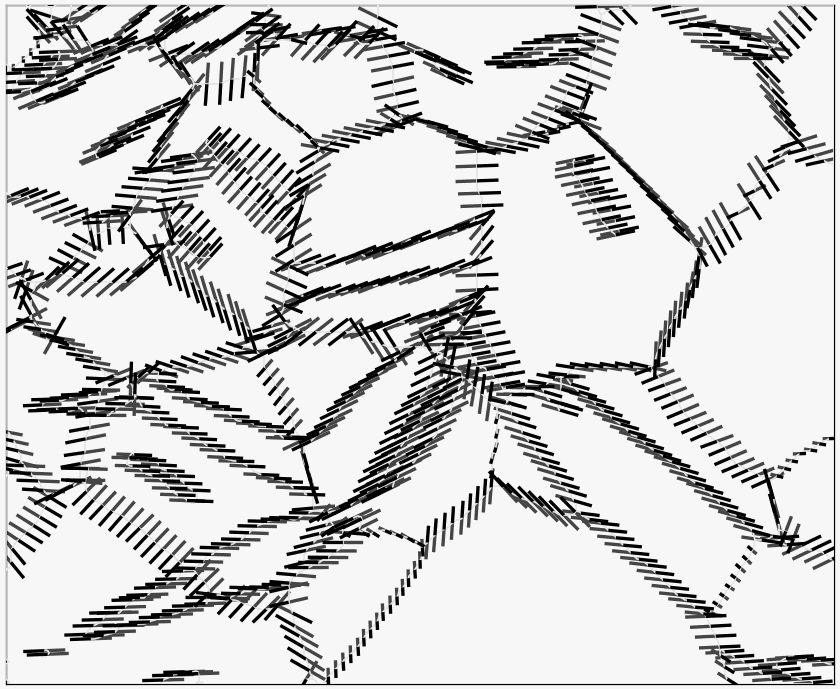
The black arrows are anchored at every third magnesium boundary midpoint. Their positions come from the boundary segments, while their directions come from the two neighbouring pixel orientations.

The same midpoint property supports spatial selection.

pos = gB_Mg.midPoint
isTop = pos.y > 30

plot(grains, faceColor=[0.9, 0.9, 0.9], faceAlpha=0.3, micronbar='off')
hold(True)
plot(gB_Mg[isTop], lineWidth=3, lineColor='red')
plot(gB_Mg[~isTop], lineWidth=3, lineColor='blue')
hold(False)

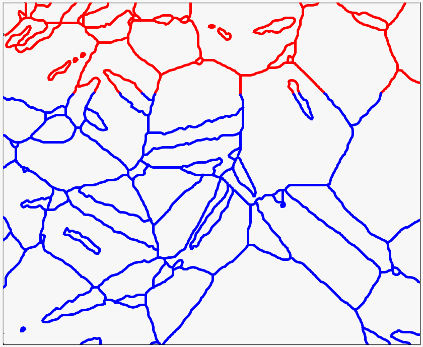
Red marks segments above \(y = 30\) micrometres, and blue marks the rest. Select Grain Boundaries develops this indexing pattern for other per-segment properties.

Two lengths are easy to confuse. len(gB_Mg) is the number of segments, whereas segLength contains the length of each segment in µm. Their sum is the total length of the selected boundary list.

totalBoundaryLength = np.sum(gB_Mg.segLength)
totalBoundaryLength

721.7001

Chains and connected components

A chain stops at a junction. A connected component does not: it contains every segment reachable through touching segments, including branches through junctions. One component can therefore contain several chains.

componentId labels each connected group. componentSize repeats the number of segments in that component on every row. It is a segment count, not a geometric length.

The next example first selects segments close to the magnesium twin relation, then colours each segment by the size of its component.

CS = ebsd.CS
twinning = orientation.map(Miller(1, -1, 0, 1, CS), Miller(1, 0, -1, -1, CS),
                           Miller(0, 1, -1, 1, CS, 'uvw'), Miller(1, -1, 0, 1, CS, 'uvw'))

gBTwin = gB[gB.isTwinning(twinning)]

plot(grains, faceColor=[0.9, 0.9, 0.9], faceAlpha=0.25, micronbar='off')
hold(True)
plot(gBTwin, gBTwin.componentSize, lineWidth=4)
hold(False)
mtexColorbar(title='segments per component')

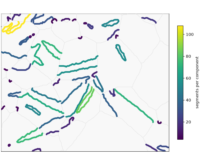
Long twin lamellae appear as large connected components. Short isolated matches appear in the low end of the colour scale and may be accidental.

numTwinComponents = np.max(gBTwin.componentId)
print(f'twin segments {len(gBTwin)}, components {numTwinComponents}')

twin segments 1648, components 54

The 1648 selected segments form 54 components. A twin lamella crossing a grain is one long component. A few isolated segments that happen to meet the twin criterion form a short component, which is why component labels are useful.

A component-scale straightness descriptor

A simple straightness descriptor divides the maximum distance between two component midpoints by the component’s total segment length. Its value approaches 1 for one straight lamella. It decreases when a component meanders or branches. This is a user-defined descriptor, not a built-in MTEX property.

componentId = gBTwin.componentId
numComponents = int(np.max(componentId))
span = np.zeros(numComponents)

for k in range(1, numComponents + 1):
  x = gBTwin.midPoint.x[componentId == k]
  y = gBTwin.midPoint.y[componentId == k]
  distanceSquared = (x - x[:, None]) ** 2 + (y - y[:, None]) ** 2
  span[k - 1] = np.sqrt(np.max(distanceSquared))

componentLength = np.bincount(componentId, gBTwin.segLength, numComponents + 1)[1:]
straightness = span / componentLength

plot(grains, faceColor=[0.9, 0.9, 0.9], faceAlpha=0.25, micronbar='off')
hold(True)
plot(gBTwin, straightness[componentId - 1], lineWidth=4)
hold(False)
mtexColorMap('blue2red')
mtexColorbar(title='component straightness')

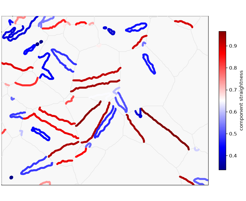
Straight components are red, while meandering or branched components are blue. The values reach 0.97 and have a median of 0.66.

Define a large component here as one containing more than 50 segments. The 13 large components have a median of 0.48, compared with 0.67 for the rest. A large component in this map is often several lamellae meeting inside one grain, rather than one long straight lamella.

componentSegmentCount = np.bincount(componentId, minlength=numComponents + 1)[1:]
isLarge = componentSegmentCount > 50
print(f'{"maximum":>10s}{"median":>10s}{"large":>8s}{"largeMedian":>14s}{"otherMedian":>14s}')
print(f'{np.max(straightness):>10.5f}{np.median(straightness):>10.5f}{np.count_nonzero(isLarge):>8d}'
      f'{np.median(straightness[isLarge]):>14.5f}{np.median(straightness[~isLarge]):>14.5f}')

   maximum    median   large   largeMedian   otherMedian
   0.96667   0.65528      13       0.48004       0.66692

This descriptor separates single straight lamellae from branched networks, rather than twins from misindexing. It is still worth checking for the latter. A few segments selected by accident, for example because of pseudosymmetry, form neither a lamella nor a branched twin network.

Next

Misorientations at Grain Boundaries develops the angle and axis on each side of a boundary. Curvature uses chain order for signed curvature, and Triple Points develops the junctions where three real grains meet.

Further reading

• V. Randle, The Measurement of Grain Boundary Geometry, Institute of Physics, 1993. This monograph connects measurable interface geometry with material properties.
• A. P. Sutton, E. P. Banks, and A. R. Warwick, The five-dimensional parameter space of grain boundaries, Proceedings of the Royal Society A 471 (2015), 20150442. It formalises the three misorientation and two boundary-plane degrees of freedom.
• G. S. Rohrer, Measuring and Interpreting the Structure of Grain-Boundary Networks, Journal of the American Ceramic Society 94 (2011), 633-646. This review connects two-dimensional boundary maps with three-dimensional interface networks.

Technical Details

grains['id', 9] addresses a grain by its id, MATLAB’s grains('id', 9). The inclusion the page follows is grain 4 inside grain 42 in MATLAB’s reconstruction and grain 9 inside grain 1 here; the two segmentations number their grains differently. ebsd['id', M] returns one measurement per entry of the matrix M, in its shape, so the two columns of ebsdId are the two sides of every segment. The two sides of a segment are its grains in the order of their ids, so the misorientation of the first segment of the inclusion runs from the host to the inclusion here and is the inverse of MATLAB’s. ebsd['id', M] lists its rows in the shape of M, row by row, where MATLAB lists the first column and then the second. componentId counts from one, so a value indexes its component’s entry at componentId - 1. MATLAB’s table is a printed line.

@article{bachmann2010mtex,
  author  = {F. Bachmann and R. Hielscher and H. Schaeben},
  title   = {Texture Analysis with MTEX - Free and Open Source Software Toolbox},
  journal = {Solid State Phenomena},
  volume  = {160},
  pages   = {63-68},
  year    = {2010},
  doi     = {10.4028/www.scientific.net/SSP.160.63},
  url     = {https://doi.org/10.4028/www.scientific.net/SSP.160.63}
}