MATLAB comes as one program. In Python the pieces come separately: Python, the language; VS Code, the editor in which you write and run your scripts; and MTEX, installed into the folder of your project. Setting them up takes about fifteen minutes. No MATLAB licence is needed.

If you already work with Python: pip install "mtex[all]" into an environment with Python 3.12 or later, and continue with step 4.

1. Install Python

Install Python 3.14 from python.org/downloads.

Windows: on the first screen of the installer, tick Add python.exe to PATH before clicking Install Now.
macOS: when the installer has finished, double-click Install Certificates.command in the Finder window that opens. Without it Python cannot download the MTEX sample data.
Linux: Python is usually there already; check with python3 --version in a terminal. On Debian and Ubuntu also run sudo apt install python3-venv.

2. Install VS Code

Install Visual Studio Code with its default settings. Start it, click the Extensions icon in the bar on the left (four small squares), and install the two extensions Python and Jupyter, both published by Microsoft. Together they let VS Code run a script piece by piece and show its figures, as the MATLAB editor does with its sections.

3. A project folder with MTEX

Make a folder for your analysis, for instance Documents/mtex-first-steps, and open it in VS Code with File > Open Folder….
Press Ctrl+Shift+P (Cmd+Shift+P on macOS), type Python: Create Environment, choose Venv and then the Python 3.14 you installed. A folder .venv appears in the file list. It holds this project’s own copy of MTEX.
Open a terminal with Terminal > New Terminal and type
```
pip install "mtex[all]" ipykernel
```
Wait until it reports Successfully installed. This downloads about 300 MB.

The environment is made once per project folder. The full description, with what to do when something goes wrong, is Installing MTEX for Python.

4. Your first script

Choose File > New File…, then Python File, and save it as first.py in the project folder. Type

# %% load a sample map
from mtex import *
ebsd = mtexdata('forsterite')
ebsd

# %% the phase map
plot(ebsd)

# %% grains and their boundaries
grains = calcGrains(ebsd['indexed'])
plot(ebsd)
hold(True)
plot(grains.boundary, lineWidth=2)
hold(False)

A line starting with # %% begins a cell, as %% begins a section in MATLAB. Click into the first cell and press Shift+Enter: the cell runs in the Interactive window that opens on the right, and the cursor moves on to the next cell. The first time, VS Code asks for a kernel; choose the one named .venv. Press Shift+Enter again for each further cell.

The Variables button in the toolbar of the interactive window lists your variables, like MATLAB’s workspace. The input box at the bottom of the interactive window works like MATLAB’s command window: type a command and press Shift+Enter.

Text after # is a comment that Python ignores. Use comments to say why a line is there; it is what you will want to know when you open the script again in half a year.

5. Open a documentation page as a script or notebook

Every page of the documentation is a script: the text you read, and the code that produced every figure on the page. In the interactive window type

openDoc('EBSDTutorial')

to write the page EBSD Tutorial into your project folder as EBSDTutorial.py and open it, or

openDoc('EBSDTutorial', notebook=True)

to get it as a Jupyter notebook, EBSDTutorial.ipynb, with the text, code and figures in one document. The name of a page is the last part of its web address without _py.html. Run it cell by cell with Shift+Enter, compare with the page, and change a number to see what it does.

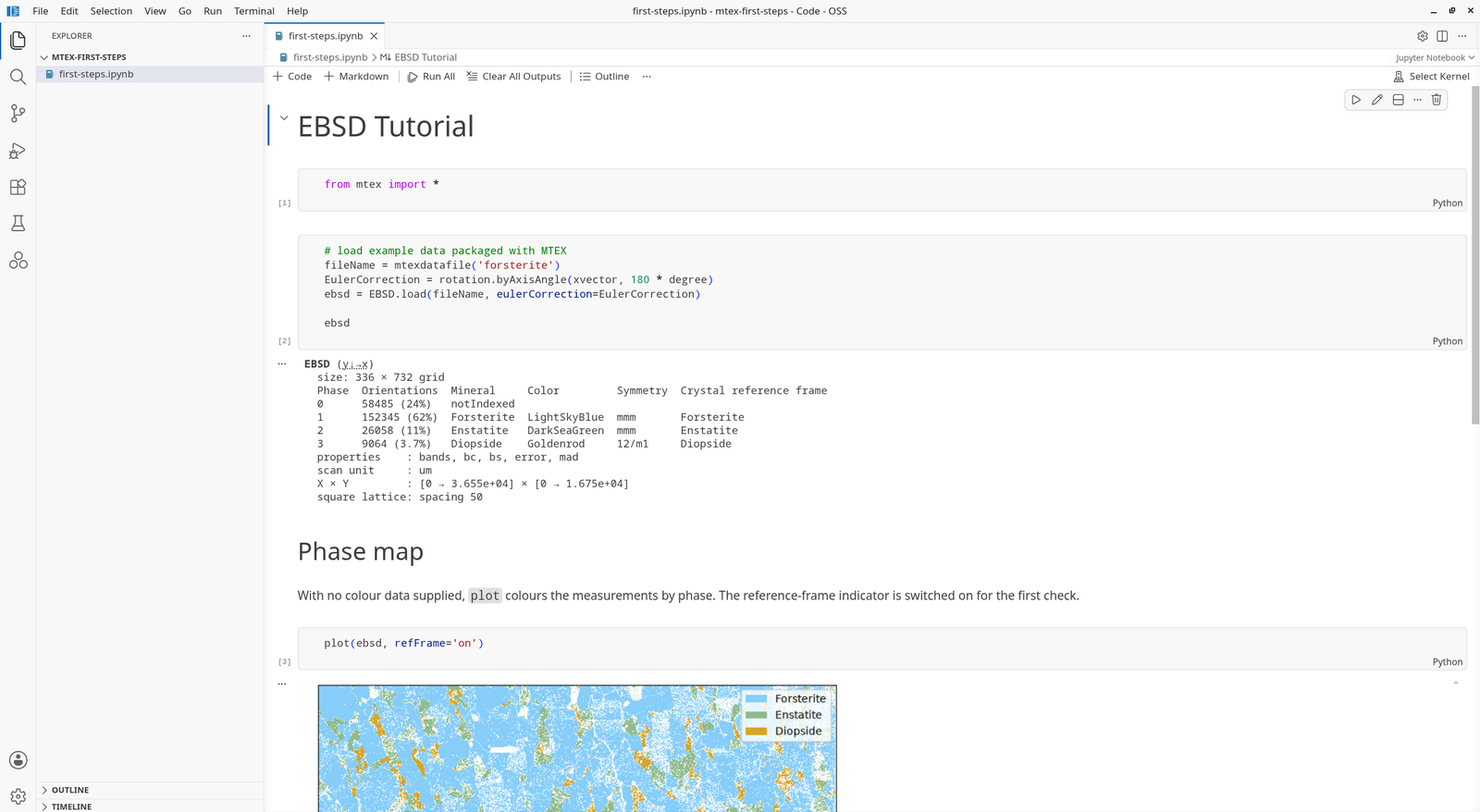
VS Code with a Jupyter notebook of the EBSD tutorial: text cells, code cells and an orientation map below the code — A documentation page opened as a notebook in VS Code.

Scripts and notebooks run the same code. A script is a plain text file, easy to compare and to keep under version control; a notebook keeps the figures next to the code, which suits exploring and sharing results.

6. Import your own data

The import wizard reads EBSD files from all common vendors. Start it from the interactive window with

ebsd = importWizard()

or, without VS Code, from a terminal with mtex-wizard.

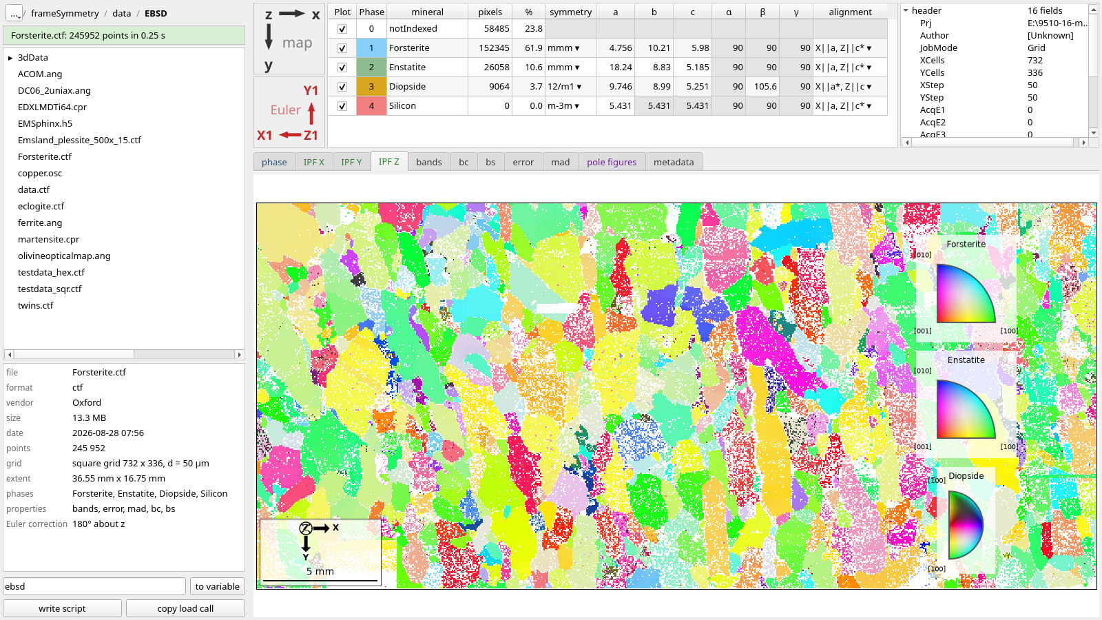
The MTEX import wizard for Python: a file browser on the left, the phase table across the top, the two coordinate systems at the top left and an orientation map below — The import wizard with an EBSD map loaded.

Browse to your data folder on the left and click a file. The wizard reads it and draws the map.
Check the phase table across the top: mineral names, symmetries and lattice parameters. Edit any cell that is wrong.
Check the two coordinate systems at the top left against your specimen: map is how the map is laid out, Euler the frame the orientations were written in. Clicking one offers the alternatives and redraws the map at once, so you can compare it with a feature you know, such as the rolling direction.
Click write script.

The wizard writes import_<file>.py into your project folder. It contains every choice you made and loads the file without the wizard; it becomes the first step of your analysis. to variable hands the data straight back to the interactive window instead, which is handy for a first look but leaves no record of how the data was read.

More on file formats and reference frames: Importing EBSD data, Importing pole figures.

7. Organise an analysis

A layout that keeps an analysis easy to rerun and to hand on:

my-steel-project/
  .venv/                    MTEX for this project
  data/                     the measured files, never edited
    sample1.ctf
  import_sample1.py         written by the import wizard
  grains_sample1.py         one script per question
  texture_sample1.ipynb     or a notebook
  results/                  figures and tables the scripts write

Keep the raw data untouched. Every correction, from cleaning to rotating the reference frame, happens in a script, so it can be checked and undone.
One import script per data set. Every analysis script starts by running it in its first cell:
```
# %%
from mtex import *
%run import_sample1.py
```
One script per question. Grain sizes in one script, texture in another. Short scripts are easier to read and to run again.
Cells for the steps. Load, clean, compute, plot, each in its own # %% cell, so you can rerun a single step while you tune it. Restart in the toolbar of the interactive window starts afresh, like MATLAB’s clear all.
Let the script write the results. With a folder results made once, saveFigure('results/grains.png') saves the current figure. A result you saved by hand cannot be reproduced.
For the next sample, copy the import script, change the file name, and run the analysis scripts again.

EBSD tutorial: from a map to grains, boundaries and texture.
Pole figure tutorial: from X-ray or neutron intensities to the ODF.
Coming from MATLAB: what changes between MATLAB and Python MTEX.
Stuck? Search or ask in the forum.

MTEX for Python, step by step