Import Pole Figure Data

A pole-figure file brings three pieces of information into one object. They are the measured specimen directions, the intensity at each direction and the lattice plane whose diffraction peak was measured. Importing is therefore more than reading a numeric table. The crystal symmetry, Miller indices and angular units have to be stated correctly. So does the specimen frame, before an ODF can be reconstructed.

MTEX stores the result in a PoleFigure object. Its entries are one or more measured pole figures, not pixels or individual orientations. The imported values are diffraction intensities. They are not yet normalized pole densities in multiples of a random distribution (mrd).

This page assumes the pole-figure idea from Pole Figures. Miller-index notation is introduced in Miller Indices. Review it if unfamiliar.

from mtex import *

Start with the import wizard

For an unfamiliar format, start the graphical wizard by entering

importWizard()

and select Pole Figure Data. The preview makes it possible to identify columns, angular units and the specimen axes before importing. The wizard can put the result in the workspace. Its more valuable output is an import script. Save that script with the analysis so the choices can be checked and the import repeated.

The wizard asks for the crystal symmetry, the Miller index of every measured reflection, and the specimen convention. These are scientific inputs, not display preferences. A plotting convention changes only where a direction is drawn. Correcting a wrong specimen frame changes what the data mean. The same distinction is explained in Reference Frames for EBSD.

A reproducible import script

The following is the essential script for the bundled Dubna quartz data. Declare the plotting convention before loading so the specimen directions enter the intended frame.

plottingConvention.default('y↑→x')

cs = crystalFrame('32', [1.4, 1.4, 1.5])

The cs definition pairs trigonal symmetry with a crystal frame. That frame holds the relative lattice parameters and interprets Miller indices. Both must describe the measured phase. The default frame is X||a*, Z||c.

# the seven Dubna files, fetched on first use; this page reads the second and the third
dubnaFiles = mtexdatafile('dubna')
fnames = [dubnaFiles[1], dubnaFiles[2]]

The two entries below correspond one for one to the two filenames. The first file measures one reflection, \((10\bar{1}0)\). The peak in the second file contains two reflections. The instrument could not resolve them, so its entry contains two Miller indices.

h = [Miller(1, 0, -1, 0, cs), Miller([[0, 1, -1, 1], [1, 0, -1, 1]], cs)]

A combined peak is a weighted sum. Its relative structure coefficients must be supplied in the same order as its Miller indices. The first pole figure has only one contribution and therefore weight 1.

c = [1, [0.52, 1.23]]

PoleFigure.load detects the file format and joins the files, reflections and weights into one object.

pf = PoleFigure.load(fnames, h, cs, superposition=c)
pf

PoleFigure (321 → y↑→x)
  h = {101̅0}, r = 72 × 19 points
  h = {011̅1}{101̅1}, r = 72 × 19 points

What was imported

The display reports the crystal symmetry and one line per measured pole figure. Here both files contain a \(72 \times 19\) grid of specimen directions. The double Miller label on the second line is deliberate. It records the superposed peak rather than pretending it was one reflection.

The four parts of the object can be inspected directly:

• pf.allH contains the crystal plane normals;
• pf.allR contains the specimen directions at which intensities were measured;
• pf.allI contains those intensities; and
• pf.c contains the structure coefficients.

The list structure matters because different pole figures may have different grids and different numbers of contributing reflections.

pf.allH

[vector3d (321)
  h  k   i  l
  1  0  -1  0, vector3d (321)
  size: 2
  h  k   i  l
  0  1  -1  1
  1  0  -1  1]

pf.c

[array([1.]), array([0.52, 1.23])]

Plot the raw measurements immediately. This catches transposed polar and azimuth columns or degrees read as radians. A flipped specimen axis and missing values are also visible. So are implausible intensity ranges, before any of them is mistaken for an ODF problem.

plot(pf)
mtexColorbar()

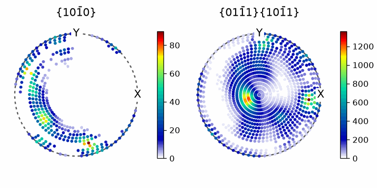
Both panels use the same \(72 \times 19\) direction grid, but their strong spots occupy different regions. The title of the second panel contains two Miller indices because it is the unresolved peak. Notice also that its raw intensity scale is much larger than the first. Raw scales must not be compared as mrd before correction and normalization.

Superposed reflections are part of the measurement model

The coefficients in pf.c are not optional cosmetic weights. For the second file the forward model used during reconstruction is the sum

Replacing that pair by one Miller index asks the inversion to explain a measured sum as a single pole figure. This generally biases the recovered ODF. If peaks overlap, record every contributing reflection. Use relative coefficients appropriate to the radiation and measured phase.

Generic text files

When no dedicated reader matches, MTEX falls back to the generic ASCII reader. A common file is one row per measurement,

polar_angle  azimuth_angle  intensity

with any number of header or unused columns. State the column meanings and positions explicitly when they cannot be inferred safely. State the angular unit as well. For example:

pf = PoleFigure.load(fname, Miller(1, 1, 1, cs), cs, interface='generic',
                     columnNames=['polar angle', 'azimuth angle', 'intensity'],
                     columns=[0, 1, 2], header=21)

The columns are counted from zero, the angles are read in degrees unless radians=True is given. Supplying the Miller index is safer than relying on a filename. A name with an unrelated number can otherwise be mistaken for a reflection. If auto-detection chooses the wrong reader, select one with interface. For example, use interface='dubna' for this format.

Supported formats and custom readers

MTEX ships readers for common text and vendor formats. The interface names of this port are dubna, siemens, geesthacht, uxd, aachen_exp, rw1 and generic. Together they cover Dubna, Siemens, Geesthacht, Bruker and Aachen data and any three column table; the PopLA, LaboTEX, BearTex, Philips, Rigaku, Juelich and PANalytical readers of MATLAB MTEX are not ported yet.

PoleFigure.load tries the installed loadPoleFigure_* readers and then the generic reader. Its reference page is version-specific. So are the reader functions in mtex/io/loadpolefigure.py.

A format-specific reader is an ordinary function, _loadPoleFigure_name by the convention of that module, that returns a PoleFigure object. Register it in the loader table of that module and call

pf = PoleFigure.load(fname, ..., interface='name')

during development. The Dubna reader in mtex/io/loadpolefigure.py is a compact format-specific template, the generic reader beside it the corresponding generic template.

Before reconstructing an ODF

Confirm the phase, lattice parameters and reflection assigned to every file. Confirm all superposition coefficients, the angular unit, specimen axes, intensity range and angular coverage. Apply only justified background, defocusing and normalization corrections. They are explained in Modify Pole Figures. Continue afterwards to ODF Reconstruction.

Further reading

• ASTM International, ASTM E81-96(2024): Standard Test Method for Preparing Quantitative Pole Figures. It distinguishes complete, partial and calculated X-ray pole figures and describes their preparation.
• D. Chateigner, L. Lutterotti and M. Morales, Quantitative texture analysis and combined analysis, International Tables for Crystallography, Volume H, chapter 5.3, 2019. It connects measured intensity, experimental corrections, normalized pole density and overlapping reflections.
• H.-J. Bunge, Texture Analysis in Materials Science: Mathematical Methods, Butterworths, English ed., 1982. It gives the classical treatment of pole figures and ODF reconstruction.

Technical Details

The sample files are fetched by mtexdatafile('dubna') on first use and kept under the data path, which is where MATLAB’s mtexDataPath points; the page picks two of the seven by position. A superposed entry is one Miller list built from a matrix with one row of four indices per reflection, where MATLAB concatenates two Miller objects. The generic reader counts its columns from zero and reads degrees by default.

@article{bachmann2010mtex,
  author  = {F. Bachmann and R. Hielscher and H. Schaeben},
  title   = {Texture Analysis with MTEX - Free and Open Source Software Toolbox},
  journal = {Solid State Phenomena},
  volume  = {160},
  pages   = {63-68},
  year    = {2010},
  doi     = {10.4028/www.scientific.net/SSP.160.63},
  url     = {https://doi.org/10.4028/www.scientific.net/SSP.160.63}
}