
Three-dimensional vectors can be added, scaled, compared, and combined. Every operation works on a whole list at once, so a loop over vectors is usually unnecessary in MTEX.
This page assumes the construction methods from Defining Three Dimensional Vectors. A reference frame is the coordinate system in which the vectors are expressed. The plotting convention below only lays that frame out on screen; it does not change the vectors.
import numpy as np
from mtex import *
plottingConvention.default('y↑→x')
Building New Vectors
Sums and multiples of the specimen axes vector3d.X, vector3d.Y, and vector3d.Z are
vector3d objects again.
v = vector3d.X + 2 * vector3d.Y
v
vector3d (y↑→x)
  x  y  z
  1  2  0
+ and - add or subtract Cartesian components. * scales a vector by a scalar. The inner product dot and cross product cross have their usual linear-algebra meanings. The order of the cross product matters.
u = dot(v, vector3d.Y) * vector3d.Y + 2 * cross(v, vector3d.Z)
u
vector3d (y↑→x)
  x  y  z
  4  0  0
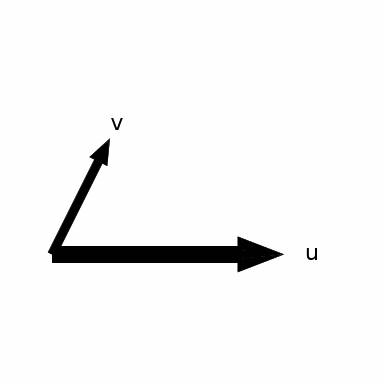
The first term is \(2\vec Y\), while the second is \(4\vec X-2\vec Y\). Their Y components cancel, leaving \(\vec u=4\vec X\). The arrows show the original vector in the XY plane and the result along positive X.
newMtexFigure()
arrow3d(v, label='v')
hold(True)
arrow3d(u, label='u')
hold(False)
Angles
The angle between two directions is a central measurement in texture analysis. One example is the tilt of a lattice-plane normal away from the sheet normal. The angle between complete crystal orientations is a different operation, introduced in Misorientations.
angle(vector3d.X, vector3d.Y) / degree
90
MTEX returns angles in radians, hence the division by degree. The angle between
directed vectors lies between \(0\) and \(180^\circ\). If the data represent axes instead,
the answer is never obtuse; see Axes and Antipodal Symmetry.
Length and Normalization
norm returns the length of each vector. normalize divides each vector by its length.
norm(u)
4
u = normalize(u)
u
vector3d (y↑→x)
  x  y  z
  1  0  0
Normalization does not change where a vector points, so it does not move its position
in a spherical plot. It matters in calculations: the dot of two unit vectors is the
cosine of their angle.
dot(normalize(v), vector3d.Y)
0.8944
A zero vector has no direction. Consequently, normalize(vector3d(0,0,0)) has undefined,
NaN components.
Lists of Vectors
cat joins vectors into one list, and an index selects an entry, the first one being
w[0]. The general rules are covered in Lists and Indexing.
w = cat(v, u)
w[0]
vector3d (y↑→x)
  x  y  z
  1  2  0
Arithmetic on a list is entry by entry. Adding the single vector v to the two-entry
list w adds it to both entries.
w = w + v
w
vector3d (y↑→x)
  size: 2
  x  y  z
  2  4  0
  2  2  0
When both inputs are lists of the same size, binary operations pair their entries by
position. The keyword outer=True of angle and
dot compares every entry of one list with every entry of
another.
Selecting from a List
The following file contains directions stored as polar and azimuth angles. Its displayed
summary confirms that the resulting vector3d list has 1,000 entries.
fname = mtexdatafile('vectors')
v = vector3d.load(fname, columnNames=['polar angle', 'azimuth angle'])
v
vector3d (y↑→x)
  size: 1000
        x       y       z
    0.174   0.984  0.0454
  0.00906   0.822   0.569
     0.43   0.901  0.0587
   -0.447  0.0187   0.894
    -0.14   0.556    0.82
        ⋮       ⋮       ⋮
    0.418   0.738    0.53
    0.205   0.196   0.959
   -0.323   0.268   0.908
   -0.249  -0.274   0.929
    0.146   0.982   0.116
A logical condition retains only directions with a polar angle below \(60^\circ\).
selected = v.theta < 60 * degree
scatter(v[selected], grid=True)
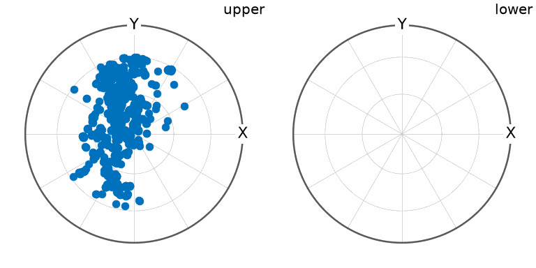
The empty outer ring shows that every plotted direction lies within \(60^\circ\) of the Z axis. Count the omitted entries directly.
numOmitted = np.sum(~selected)
numOmitted
236
Thus, 236 of the 1,000 directions lie at least \(60^\circ\) away from the Z axis.
Averaging a List
mean averages the Cartesian components. The result is a mean vector, which generally is not a unit vector.
m = mean(v)
m
vector3d (y↑→x)
       x      y      z
  -0.137  0.198  0.677
Normalizing it gives the mean direction.
meanDirection = normalize(m)
meanDirection
vector3d (y↑→x)
      x      y      z
  -0.19  0.276  0.942
Because every input vector has unit length, the length of m is the mean resultant
length.
meanResultantLength = norm(m)
meanResultantLength
0.7186
Here it is about 0.719. Identical unit directions give one; dispersed or mutually cancelling directions give a shorter result. Normalize unequal input vectors first when this directional statistic is intended.
Opposite directed observations cancel. For axes, where v and -v mean the same thing,
use mean(v, antipodal=True) instead; see
Axes and Antipodal Symmetry.
Operations at a Glance
These methods operate elementwise unless their description says otherwise.
| angle(v1,v2) | pointwise angle between vectors |
| angle(v1,v2,outer=True) | all pairwise angles |
| dot(v1,v2) | pointwise inner product |
| dot(v1,v2,outer=True) | all pairwise inner products |
| cross(v1,v2) | pointwise cross product |
| a*v | multiplication by a scalar |
| a*v | componentwise scaling by an array of the same size |
| norm(v) | length of every vector |
| normalize(v) | length scaled to one |
| orth(v) | an arbitrary orthogonal unit vector |
| orthProj(v,N) | component orthogonal to N |
| perp(v) | best-fit direction orthogonal to a list |
| v.sum() | componentwise sum over a list |
| mean(v) | mean vector, or mean axis for antipodal data |
| polar(v) | polar angle, azimuth, and length |
| rotate(v,rot) | turn by a rotation |
Further Reading
- N. I. Fisher, T. Lewis, and B. J. J. Embleton, Descriptive and ancillary methods, and sampling problems, in Statistical Analysis of Spherical Data, Cambridge University Press, 1987, treats mean directions, resultant lengths, and the difference between vectorial and axial data.
Next
Density Estimation replaces a long list of directions by a smooth function on the sphere. Read Axes and Antipodal Symmetry before analysing data whose two signs are physically equivalent. Turning a direction into another one is the job of a rotation.
Citing this page.
This page is part of the documentation of
MTEX, a free and open
source MATLAB toolbox for analyzing and modeling crystallographic textures.
It was written by The MTEX Developers and is published at
https://mtex-toolbox.github.io/VectorsOperations_py.html.
If you use MTEX, or reuse text or figures from this page, in your research,
please cite
F. Bachmann, R. Hielscher, H. Schaeben: Texture Analysis with MTEX - Free and Open Source Software Toolbox, Solid State Phenomena 160 (2010), 63-68. 10.4028/www.scientific.net/SSP.160.63
BibTeX
@article{bachmann2010mtex,
  author  = {F. Bachmann and R. Hielscher and H. Schaeben},
  title   = {Texture Analysis with MTEX - Free and Open Source Software Toolbox},
  journal = {Solid State Phenomena},
  volume  = {160},
  pages   = {63-68},
  year    = {2010},
  doi     = {10.4028/www.scientific.net/SSP.160.63},
  url     = {https://doi.org/10.4028/www.scientific.net/SSP.160.63}
}
Other papers describing specific MTEX methods are listed under Publications — please cite the one that best fits your application. The MTEX source code is licensed under the GNU General Public License v2.0; the text and figures of this documentation are licensed under CC BY 4.0, which permits reuse — including by automated systems — provided The MTEX Developers and this page are credited.