Changing Crystal-Axis Settings

A crystal-axis setting assigns the names \(\vec a\), \(\vec b\) and \(\vec c\) to physical lattice vectors. A crystal frame is the Cartesian reference frame glued to that labelled lattice basis. It is distinct from the point group attached to it and from the plotting convention used to draw it.

This page assumes the direct and reciprocal axes introduced in Miller Indices. Read The Crystal Reference System first if the Cartesian embedding of a non-orthogonal lattice is new to you.

Two kinds of convention occur in published data. One source may keep the same lattice labels but embed them in a different Cartesian crystal frame. Another may rename or permute the lattice axes themselves. Both change numerical coordinates, so both require an explicit frame change in MTEX.

import numpy as np

from mtex import *

plottingConvention.default('y↑→x')

Read the Crystal Frame from the Summary

crystalFrame stores the point group, lattice metric and crystal frame together. Its printed summary is therefore the first place to check a convention. For this monoclinic example, MTEX uses \(\vec x\parallel\vec a^*\) and \(\vec z\parallel\vec c\) by default.

cs = crystalFrame('12/m1', [4, 5, 6], np.array([90, 100, 90]) * degree, mineral='example')
cs

crystalFrame (⊙c*→b)
  mineral           : example
  symmetry          : 12/m1
  elements          : 4
  a, b, c           : 4, 5, 6
  alpha, beta, gamma: 90°, 100°, 90°
  reference frame   : X||a*, Y||b, Z||c

The summary reports X||a*, Y||b, Z||c. The direct axis \(\vec a\) is \(10^\circ\) from \(\vec x\), while the reciprocal axis \(\vec a^*\) is parallel to it. The symmetry=False option asks for these geometric angles without replacing either direction by a symmetry-equivalent one.

axisAngles = np.array([angle(cs.aAxis, vector3d.X, symmetry=False), angle(cs.aAxisRec, vector3d.X, symmetry=False)]) / degree
axisAngles

array([10.,  0.])

A different Cartesian embedding is requested by naming the parallel axes in the constructor.

csAlternative = crystalFrame('12/m1', [4, 5, 6], np.array([90, 100, 90]) * degree, 'X||a', mineral='example')
csAlternative

crystalFrame (⊙c*→b)
  mineral           : example
  symmetry          : 12/m1
  elements          : 4
  a, b, c           : 4, 5, 6
  alpha, beta, gamma: 90°, 100°, 90°
  reference frame   : X||a, Y||b, Z||c*

The second summary reports X||a, Y||b, Z||c*. The point group and lattice metric have not changed, but Miller indices, Euler angles and tensor components now refer to a different crystal frame. This is the embedding convention developed on the preceding page.

A Published Axis Permutation

A separate problem arises when two sources assign the labels \(\vec a\), \(\vec b\) and \(\vec c\) to different physical lattice vectors. The bundled data file contains the room-pressure stiffness tensor of San Carlos olivine measured by Abramson et al. (1997). Its source setting has lattice lengths \(a=4.7646\), \(b=10.2296\) and \(c=5.9942\), with tensor axes \(X_1\parallel[100]\) and \(X_3\parallel[001]\).

csSource = crystalFrame('mmm', [4.7646, 10.2296, 5.9942], mineral='Olivine')
fname = mtexdatafile('olivine1997')
C = stiffnessTensor.load(fname, csSource)
C

stiffnessTensor (Olivine)
  density: 3.355
  unit   : GPa
  rank   : 4 (3 × 3 × 3 × 3)
  tensor in Voigt matrix representation
  320.5  68.15   71.6   0   0     0
  68.15  196.5   76.8   0   0     0
   71.6   76.8  233.5   0   0     0
      0      0      0  64   0     0
      0      0      0   0  77     0
      0      0      0   0   0  78.7

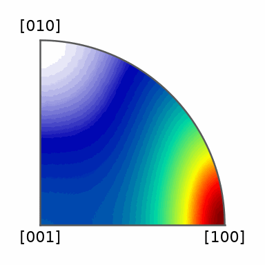
The printed Voigt matrix is useful here because its components are the quantities that a frame change must rewrite. The plot below shows the directional magnitude \(C_{ijkl}n_i n_j n_k n_l\). It is a compact view of the component permutation, not Young’s modulus or a complete elastic response.

plot(C)

Suppose the target convention cyclically renames the axes: old \(\vec b\) becomes new \(\vec a\), old \(\vec c\) becomes new \(\vec b\), and old \(\vec a\) becomes new \(\vec c\). The reordered lattice lengths state that mapping.

csTarget = crystalFrame('mmm', [10.2296, 5.9942, 4.7646], mineral='Olivine')
csTarget

crystalFrame (⊙c→a)
  mineral : Olivine
  symmetry: mmm
  elements: 8
  a, b, c : 10.23, 5.994, 4.765

Change the Frame, Do Not Rotate the Tensor

A frame change re-expresses the same physical object in another reference frame. It does not move the object. For a tensor, transformReferenceFrame applies the required basis change to every component and attaches the target crystal frame.

CTarget = C.transformReferenceFrame(csTarget)
CTarget

stiffnessTensor (Olivine)
  density: 3.355
  unit   : GPa
  rank   : 4 (3 × 3 × 3 × 3)
  tensor in Voigt matrix representation
  196.5   76.8  68.15   0     0   0
   76.8  233.5   71.6   0     0   0
  68.15   71.6  320.5   0     0   0
      0      0      0  77     0   0
      0      0      0   0  78.7   0
      0      0      0   0     0  64

nextAxis()
plot(CTarget)

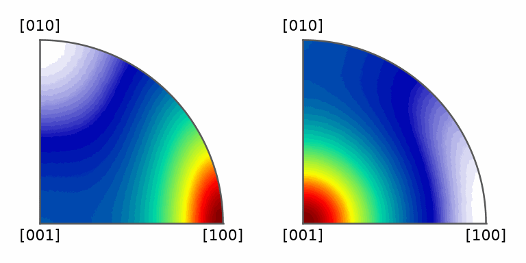
In the left panel, the red maximum is labelled \([100]\). In the right panel, the same feature is labelled \([001]\) because old \(\vec a\) is new \(\vec c\). The feature has not rotated in the material; only its coordinates and crystallographic label have changed.

The directional value along that physical axis is unchanged. The source direction \([100]\) and the target direction \([001]\) both give 320.5 GPa.

sourceA = Miller(1, 0, 0, csSource, 'uvw')
targetC = Miller(0, 0, 1, csTarget, 'uvw')
sameDirectionalValue = np.array([C.directionalMagnitude(sourceA), CTarget.directionalMagnitude(targetC)])
sameDirectionalValue

array([320.5, 320.5])

Avoid Three Common Mistakes

Do not attach csTarget to the unmodified component matrix. That would describe a different physical tensor. Use rotate only when the material property itself moves; use transformReferenceFrame when only its coordinates change.

Do not infer an axis mapping by sorting lattice lengths. Record the old and new basis relation from the data source, including axis signs and handedness. Some point groups also have setting-specific symbols, such as 2mm, m2m and mm2; see Crystal Symmetries.

Finally, a plotting convention only lays a reference frame out on screen. Changing it cannot repair a wrong crystal frame. When importing a tensor, also record its units and compact-matrix convention; the complete audit is developed in Importing Tensor Data. Orientations use the analogous transformReferenceFrame method.

Further Reading

• H. Arnold, Transformations of the coordinate system (unit-cell transformations), International Tables for Crystallography A, ch. 5.1, 2006, gives basis-change matrices for conventional crystallographic settings.
• J. F. Nye, Physical Properties of Crystals: Their Representation by Tensors and Matrices, Oxford University Press, 1985, develops tensor components and changes of Cartesian axes.
• D. Rowenhorst et al., Consistent representations of and conversions between 3D rotations, Modelling and Simulation in Materials Science and Engineering 23, 083501, 2015, explains why crystal and specimen frame conventions must be stated explicitly.
• E. H. Abramson, J. M. Brown, L. J. Slutsky and J. Zaug, The elastic constants of San Carlos olivine to 17 GPa, Journal of Geophysical Research 102(B6), 12253-12263, 1997, is the source of the stiffness tensor used above.

Next

Crystal Shapes continues the chapter by drawing indexed crystal faces. Importing Tensor Data applies this frame audit to component tables, and Importing Orientations applies it to orientation files.

Technical Details

The tensor file of the MATLAB data folder is the sample data set olivine1997 here, fetched on first use; mtexdatafile gives its path for stiffnessTensor.load.

@article{bachmann2010mtex,
  author  = {F. Bachmann and R. Hielscher and H. Schaeben},
  title   = {Texture Analysis with MTEX - Free and Open Source Software Toolbox},
  journal = {Solid State Phenomena},
  volume  = {160},
  pages   = {63-68},
  year    = {2010},
  doi     = {10.4028/www.scientific.net/SSP.160.63},
  url     = {https://doi.org/10.4028/www.scientific.net/SSP.160.63}
}