Convolution of Rotational and Spherical Functions

Convolution combines two functions by averaging their overlap while one argument is rotated. It is used to smooth a function, transfer an orientation distribution to directions, and construct rotation-dependent similarities. A cross-correlation uses the same machinery but may also require inversion or complex conjugation, depending on its convention.

Four combinations occur in MTEX:

The left and right sides are defined on Symmetry of Orientation-Dependent Functions. Matching means the same point group in the same reference frame, not merely point groups with the same printed name.

import numpy as np

from mtex import *

plottingConvention.default('y↑→x')

Convolve two rotational functions

The inner sides are integrated out. Consequently, the right symmetry of the first function must match the left symmetry of the second. The result inherits its left symmetry from the first function and its right symmetry from the second.

rng = np.random.default_rng(1)
g = SO3FunHarmonic.example()

ss1 = specimenFrame()
ss2 = specimenFrame('222')
centre = orientation.rand(1, ss1, ss2, rng=rng)
kernel = SO3DeLaValleePoussinKernel(halfwidth=15 * degree)
f = SO3FunRBF(centre, kernel)

c = conv(f, g)
c

SO3FunHarmonic (Quartz → y↑→x)
  bandwidth: 17
  mean     : 1

resultLeftSymmetry = c.frameB
resultLeftSymmetry

specimenFrame (specimen, y↑→x)
  symmetry: 222
  elements: 4

resultRightSymmetry = c.frameA
resultRightSymmetry

crystalFrame (⊙c→a)
  mineral        : Quartz
  symmetry       : 321
  elements       : 6
  a, b, c        : 4.916, 4.916, 5.405
  reference frame: X||a*, Y||b, Z||c

Here f.frameA and g.frameB are both the identity specimen symmetry. The result therefore keeps the 222 left symmetry of f and the quartz right symmetry of g.

Check one value against direct numerical integration. The SO3Fun mean uses normalized orientation-space measure, so it implements the factor \(1/(8\pi^2)\) in the integral stated below.

r = orientation.rand(c.CS, c.SS, rng=rng)
convolutionValue = c.eval(r)
integrand = SO3FunHandle(lambda q: f.eval(rotation(q)) * g.eval(inv(rotation(q)) * r))
integralValue = mean(integrand, resolution=5 * degree)
SO3CheckDifference = abs(convolutionValue - integralValue)
print(f'convolution {convolutionValue:.4f}, integral {integralValue:.4f}, difference {SO3CheckDifference:.4f}')

convolution 0.7023, integral 0.7041, difference 0.0018

plot(c, 'sigma')

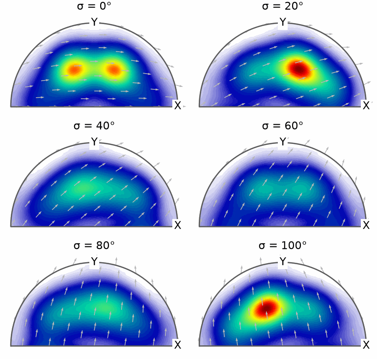
The strongest regions are shifted and broadened copies of the input ODF. The maximum drops from about 94 to about 10, the bandwidth from 48 to 17, and the peak moves.

The plot covers the fundamental region of the inherited 222 and quartz symmetries, so symmetrically equivalent copies are folded into it rather than drawn beside one another. The printed difference measures the accuracy of the independent, coarser numerical integration used for the check.

Swap the argument order

Convolution on the rotation group is not commutative in general. A right-sided form can be evaluated by swapping the function order, provided the new inner symmetry pair is compatible.

rng = np.random.default_rng(3)
fRight = SO3FunRBF(orientation.rand(1, g.CS, g.CS, rng=rng), kernel)
cRight = conv(g, fRight)
cRight

SO3FunHarmonic (Quartz → y↑→x)
  bandwidth: 17
  mean     : 1

rRight = orientation.rand(cRight.CS, cRight.SS, rng=rng)
rightConvolutionValue = cRight.eval(rRight)
qRight = orientation.rand(100000, fRight.frameA.stripSym(), fRight.frameB.stripSym(), rng=rng)
rightSamples = fRight.eval(qRight) * g.eval(rRight * inv(qRight))
rightIntegralEstimate = np.mean(rightSamples)
rightStandardError = np.std(rightSamples, ddof=1) / np.sqrt(rightSamples.size)
rightCheckDifference = abs(rightConvolutionValue - rightIntegralEstimate)
print(f'convolution {rightConvolutionValue:.4f}, estimate {rightIntegralEstimate:.4f}, '
      f'standard error {rightStandardError:.4f}, difference {rightCheckDifference:.4f}')

convolution 0.1909, estimate 0.1928, standard error 0.0018, difference 0.0019

This Monte Carlo estimate checks the right-sided integral written in the maths section. Compare its difference with the printed standard error. It is not a claim that conv(f, g) and conv(g, f) are generally equal.

Arrays of SO3Fun objects may also be convolved. Two arrays are combined element by element, as described for vector-valued rotational functions.

Convolve two spherical functions

Rotating one spherical function against another produces a function of the rotation, not another spherical function. The output measures their overlap for every relative orientation. Its right symmetry comes from the first spherical function and its left symmetry from the second.

cs = crystalFrame()
sphereF = S2FunHarmonic(S2Fun.smiley(), cs)
sphereG = S2FunHarmonic(S2DeLaValleePoussinKernel())
sphereCorrelation = conv(sphereF, sphereG)
sphereCorrelation

SO3FunHarmonic (1 → y↑→x)
  bandwidth: 25
  mean     : 0.006417

rSphere = orientation.rand(sphereCorrelation.CS, sphereCorrelation.SS, rng=rng)
sphereConvolutionValue = sphereCorrelation.eval(rSphere)
sphereIntegrand = S2FunHandle(lambda v: sphereF.eval(inv(rSphere) * v) * sphereG.eval(v))
sphereGrid = equispacedS2Grid(resolution=1 * degree)
sphereIntegralValue = np.mean(sphereIntegrand.eval(sphereGrid))
sphereCheckDifference = abs(sphereConvolutionValue - sphereIntegralValue)
print(f'convolution {sphereConvolutionValue:.4e}, integral {sphereIntegralValue:.4e}, difference {sphereCheckDifference:.2e}')

convolution -1.1909e-06, integral -1.1123e-06, difference 7.86e-08

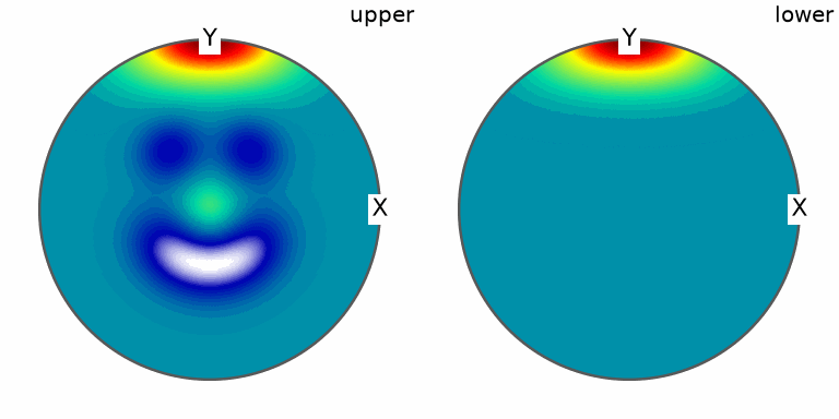
plot(sphereCorrelation, 'sigma')

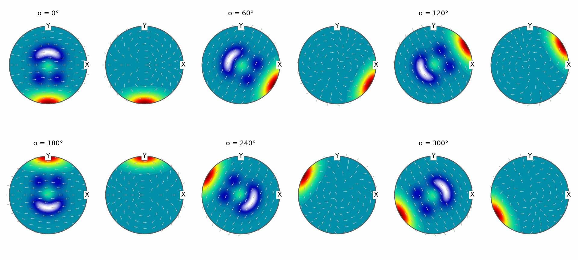
The section plot changes as the smiley pattern moves into and out of alignment with the zonal second function. This is why two inputs on the sphere produce an output on the rotation group.

Convolve a rotational and a spherical function

A rotational function can transport a spherical function through all orientations and average the result. The output is spherical. The spherical symmetry must match the left symmetry of the rotational function, and the output inherits the rotational function’s right symmetry.

rotF = SO3FunHarmonic.example()
sphereH = S2FunHarmonic(S2Fun.smiley(), rotF.frameB)
directionF = conv(rotF, sphereH)
directionF

S2FunHarmonic (Quartz)
  bandwidth: 48
  mean     : 0.006417

vCrystal = Miller(1, 0, 0, directionF.frame)
directionValue = directionF.eval(vCrystal)

rng = np.random.default_rng(7)
qDirection = orientation.rand(100000, rotF.CS.stripSym(), rotF.frameB, rng=rng)
directionSamples = rotF.eval(qDirection) * sphereH.eval(qDirection * vCrystal)
directionIntegralEstimate = np.mean(directionSamples)
directionStandardError = np.std(directionSamples, ddof=1) / np.sqrt(directionSamples.size)
directionCheckDifference = abs(directionValue - directionIntegralEstimate)
print(f'convolution {directionValue:.4f}, estimate {directionIntegralEstimate:.4f}, '
      f'standard error {directionStandardError:.4f}, difference {directionCheckDifference:.4f}')

convolution 0.0342, estimate 0.0340, standard error 0.0014, difference 0.0002

plot(directionF)

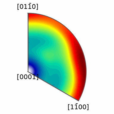
Bright directions receive large contributions from many orientations where both input functions are large. Unlike the preceding section plot, this result needs only a direction on the sphere for evaluation.

The Monte Carlo orientations cover the full rotation group. stripSym removes the quartz point group while retaining its crystal frame. Using a symmetry-reduced fundamental region would be invalid for this check, because a fixed Miller representative makes the integrand nonsymmetric. The check difference should be interpreted against its sampling standard error, not as deterministic quadrature error.

Use the inverse-action variant

A second convention acts on the spherical argument with the inverse rotation. It applies when the rotational function has trivial left symmetry and its right symmetry matches the spherical symmetry. Add 'inv', or equivalently invert the rotational function before calling conv.

sphereHInv = S2FunHarmonic(S2Fun.smiley(), rotF.CS)
directionInv = conv(rotF, sphereHInv, inverse=True)
directionInvEquivalent = conv(inv(rotF), sphereHInv)

vSpecimen = xvector
inverseActionValue = directionInv.eval(vSpecimen)

rng = np.random.default_rng(5)
qInverse = orientation.rand(100000, rotF.CS.stripSym(), rotF.frameB, rng=rng)
inverseSamples = rotF.eval(qInverse) * sphereHInv.eval(inv(qInverse) * vSpecimen)
inverseIntegralEstimate = np.mean(inverseSamples)
inverseStandardError = np.std(inverseSamples, ddof=1) / np.sqrt(inverseSamples.size)
inverseActionCheckDifference = abs(inverseActionValue - inverseIntegralEstimate)
print(f'convolution {inverseActionValue:.4f}, estimate {inverseIntegralEstimate:.4f}, '
      f'standard error {inverseStandardError:.2e}, difference {inverseActionCheckDifference:.2e}')

convolution 0.0148, estimate 0.0148, standard error 3.18e-04, difference 7.30e-05

comparisonGrid = equispacedS2Grid(resolution=5 * degree)
inverseFlagDifference = np.max(np.abs(directionInv.eval(comparisonGrid) - directionInvEquivalent.eval(comparisonGrid)))
inverseFlagDifference

0

The small final difference verifies that 'inv' and conv(inv(rotF), sphereHInv) implement the same variant. The two action conventions should not be mixed: \(qv\) and \(q^{-1}v\) generally produce different averages.

Smooth with a rotational kernel

An SO3Kernel is a radial rotational function: it depends only on the rotation angle. Convolution with it attenuates harmonic degrees according to the kernel coefficients. Radiality also makes this particular convolution commutative, even though convolution of two general rotational functions is not.

psi = SO3DeLaValleePoussinKernel(halfwidth=10 * degree)
smoothSource = SO3FunHarmonic(rotF, bandwidth=min(rotF.bandwidth, psi.bandwidth))
smoothF = conv(smoothSource, psi)
smoothFReverse = conv(psi, smoothSource)
kernelCommutationError = calcError(smoothF, smoothFReverse)
kernelCommutationError

0

plotSpectrum([smoothSource, smoothF], figSize='small')
legend('before convolution', 'after convolution')

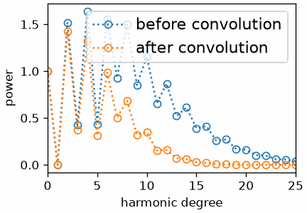
The convolved spectrum lies below the original at higher harmonic degrees. Those degrees encode rapid angular variation, so their attenuation is the spectral signature of smoothing.

Smooth with a spherical kernel

An S2Kernel is a zonal spherical function. Convolving an S2Fun with it produces another S2Fun and smooths angular variation around every direction.

sphericalSource = S2Fun.smiley()
phi = S2DeLaValleePoussinKernel(halfwidth=10 * degree)
sphericalSmooth = conv(sphericalSource, phi)
sphericalSmooth

S2FunHarmonic
  bandwidth: 25
  mean     : 0.006417

plot(sphericalSmooth)

The face remains recognizable, while the sharp boundaries of its features are softened by the 10 degree kernel.

The same kernel can be regarded as a spherical function and convolved with sphericalSource to produce an SO3Fun. The two results agree when the direction \(v\) and rotation \(R\) satisfy \(v=R^{-1}e_3\).

v = vector3d.rand(rng=rng)
rKernel = rotation.map(v, zvector)
kernelAsFunction = S2FunHarmonic(phi)
sphericalOnSO3 = conv(sphericalSource, kernelAsFunction)
kernelFormDifference = abs(sphericalSmooth.eval(v) - sphericalOnSO3.eval(rKernel))
kernelFormDifference

8.3267e-17

xi = equispacedS2Grid(resolution=1 * degree)
sphericalKernelIntegral = np.mean(sphericalSource.eval(xi) * phi.eval(np.cos(angle(xi, v))))
sphericalKernelCheckDifference = abs(sphericalSmooth.eval(v) - sphericalKernelIntegral)
print(f'integral {sphericalKernelIntegral:.4f}, difference {sphericalKernelCheckDifference:.2e}')

integral 0.1779, difference 4.64e-05

The maths behind convolution

MTEX uses normalized Haar measure. If \(\mathrm{d}q\) denotes the usual unnormalized measure with volume \(8\pi^2\), convolution of compatible rotational functions is

If \(f\) has left symmetry \(S_L\) and right symmetry \(S_x\), while \(g\) has left symmetry \(S_x\) and right symmetry \(S_R\), the result has left symmetry \(S_L\) and right symmetry \(S_R\). Swapping the order gives the right-sided form

The sphere has volume \(4\pi\). For two spherical functions, MTEX uses

The two rotational–spherical actions are

and, with 'inv',

Finally, a zonal spherical kernel \(\psi\) satisfies

Regarding the kernel as the spherical function \(\psi(\xi\mathbin{\cdot}e_3)\) instead gives an SO3Fun. Its value at \(R\) equals the spherical result at \(v=R^{-1}e_3\). For an SO3Kernel, \(\omega(q^{-1}R)=\omega(Rq^{-1})\) explains the special commutativity.

References

• P. J. Kostelec and D. N. Rockmore, FFTs on the rotation group, Journal of Fourier Analysis and Applications 14 (2008), 145–179, develops the Fourier transform on \(\mathrm{SO}(3)\) that turns convolution into multiplication of Wigner coefficient matrices.
• H.-J. Bunge, Texture Analysis in Materials Science: Mathematical Methods, Butterworths (1982), gives the harmonic framework for ODFs, pole figures, and their rotational integral operators.

Next

Continue with Vector-Valued Functions to apply the elementwise array behaviour introduced above. The following Rotational Vector Fields page extends the domain to vector-valued fields with a rotating tangent space.

Technical Details

MATLAB’s S2FunHarmonicSym(sF, cs) is S2FunHarmonic(sF, cs) here, a function in the frame of its symmetry; the random draws are NumPy’s, so the checks agree with MATLAB’s in kind, not in their digits. MATLAB’s smoothSource = rotF; smoothSource.bandwidth = … copies the function; the page builds the truncated copy with the constructor, since the Python assignment would change rotF itself.

@article{bachmann2010mtex,
  author  = {F. Bachmann and R. Hielscher and H. Schaeben},
  title   = {Texture Analysis with MTEX - Free and Open Source Software Toolbox},
  journal = {Solid State Phenomena},
  volume  = {160},
  pages   = {63-68},
  year    = {2010},
  doi     = {10.4028/www.scientific.net/SSP.160.63},
  url     = {https://doi.org/10.4028/www.scientific.net/SSP.160.63}
}