Fourier Series on the Circle

A function on the circle assigns a value to an in-plane angle \(\rho\). Its values repeat after \(2\pi\), so it is a \(2\pi\)-periodic function. Geometrically, its domain is also called the one-dimensional sphere \(\mathbb{S}^1\) or the one-dimensional torus.

The preceding Spherical Harmonics page introduced wave-like basis functions on the sphere. On the circle, only one integer mode remains, and the corresponding expansion is an ordinary Fourier series.

MTEX uses functions on the circle whenever a scalar quantity depends on an in-plane angle. Typical examples are

• angular density distributions of grain long axes or other in-plane shape directions,
• distributions of grain-boundary segment directions, optionally weighted by their segment lengths,
• caliper and projection lengths as functions of the projection direction, and
• azimuth-angle distributions of three-dimensional directions.

Start from an explicit formula

MTEX offers two complementary representations. An S1FunHandle evaluates an explicit formula whenever a value is requested. An S1FunHarmonic stores a finite set of Fourier coefficients.

Begin with the formula

Pass the Python function to S1FunHandle.

import matplotlib.pyplot as plt
import numpy as np

from mtex import *

S1F = S1FunHandle(lambda rho: 1 + 0.5 * np.cos(2 * rho))
S1F

S1FunHandle
  bandwidth hint: 1024

Plot the same function in two ways

A polar plot places each value along its angle. A Cartesian plot unfolds the circle and shows angle on the horizontal axis.

plt.figure()
plt.subplot(1, 2, 1, projection='polar')
plot(S1F, lineWidth=2)
mtexTitle('Polar Plot')
plt.subplot(1, 2, 2)
plot(S1F, lineWidth=2, polar=False)
mtexTitle('Cartesian Plot')

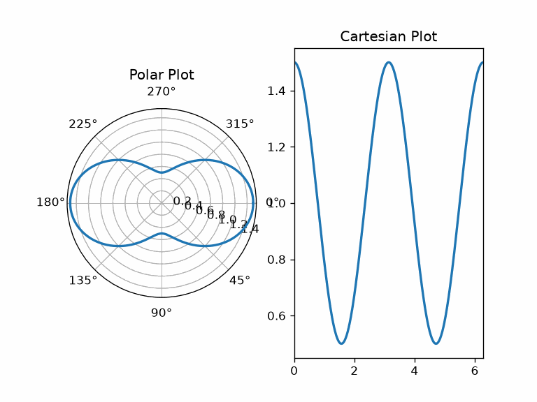
Read the two views

The Cartesian view makes the two maxima over one full turn easy to count. The polar view makes their opposite in-plane directions visible. Both panels show the same function, and neither changes its representation.

Construct a function from coefficients

Within S1FunHarmonic, the fhat property stores coefficients from mode \(-N\) through mode \(N\). It therefore contains an odd number of entries, and the centre entry is the constant mode.

As an example, the following Fourier coefficients describe the real-valued function \(f(\rho)=4+\cos\rho+2\sin(2\rho)\).

fhat = [-1j, 0.5, 4, 0.5, 1j]
S1FCoeff = S1FunHarmonic(fhat)
S1FCoeff

S1FunHarmonic
  bandwidth: 2
  mean     : 4

coefficientMean = mean(S1FCoeff)
coefficientMean

4

plt.figure()
plt.subplot(1, 2, 1, projection='polar')
plot(S1FCoeff, lineWidth=2)
mtexTitle('Polar Plot')
plt.subplot(1, 2, 2)
plot(S1FCoeff, lineWidth=2, polar=False)
mtexTitle('Cartesian Plot')

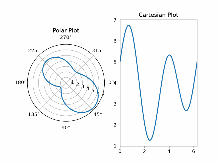
Read the coefficient example

The two coefficients of magnitude \(0.5\) form the cosine term. The outer imaginary coefficients form the sine term. A real-valued function has conjugate coefficients in opposite modes.

The centre entry is the mean value. In the vector as written it is 4, which is confirmed by coefficientMean.

Approximate a formula by a Fourier series

Constructing an S1FunHarmonic from an S1FunHandle computes the Fourier coefficients. The bandwidth is the largest retained mode. A higher bandwidth generally improves the approximation but also increases the computational cost.

Computations with bandwidth 1024 are still very fast in practice and usually provide a good approximation. The much smaller bandwidth 20 is already sufficient for the smooth function below.

S1F = S1FunHandle(lambda rho: np.exp(np.cos(rho)))
S1FH = S1FunHarmonic(S1F, bandwidth=20)
S1FH

S1FunHarmonic
  bandwidth: 20
  mean     : 1.266

rhoCheck = np.linspace(0, 2 * np.pi, 1001)
maxApproximationError = np.max(np.abs(S1F.eval(rhoCheck) - S1FH.eval(rhoCheck)))
maxApproximationError

2.5313e-14

plot(S1F, lineWidth=2)
hold(True)
plot(S1FH, '--', lineWidth=2)
hold(False)
legend('S1FunHandle', 'S1FunHarmonic')

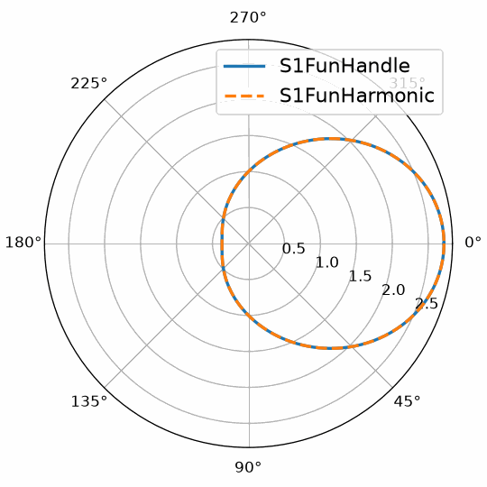
Read the approximation

The solid formula and dashed Fourier approximation overlap throughout the circle. The printed maximum error on the check grid is about \(10^{-14}\), so the remaining difference is at the scale of floating-point round-off.

Fit values sampled at angles

A function is often known only at a finite set of angles. S1FunHarmonic.interpolate constructs a periodic trigonometric polynomial from those samples. The result can be evaluated at arbitrary angles, plotted, differentiated, or used in later computations.

The bandwidth sets the number of Fourier modes in the interpolation. It should be large enough to resolve the measured angular variation. An unnecessarily large bandwidth can introduce oscillations or amplify noise.

rho = np.linspace(0, 2 * np.pi, 11)
values = 1 + np.cos(rho) + 2 * np.sin(2 * rho)

S1FI = S1FunHarmonic.interpolate(rho, values)
S1FI

S1FunHarmonic
  bandwidth: 3
  mean     : 1

sampleResidual = np.max(np.abs(S1FI.eval(rho) - values))
sampleResidual

3.4361e-04

plt.figure()
plt.plot(rho, values, 'x', label='samples')
hold(True)
plot(S1FI, lineWidth=2, polar=False, displayName='periodic fit')
hold(False)
legend()

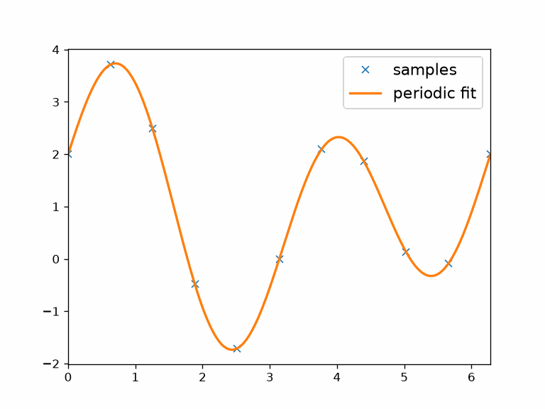
Read the sampled-data fit

The curve joins the angular trend and closes periodically between \(2\pi\) and zero. The default regularisation leaves a maximum residual of about \(3.4\cdot10^{-4}\) at these samples. Set bandwidth and regularisation deliberately when the data contain noise or sharp changes.

Smooth small-scale oscillations

A harmonic function obtained from measured or interpolated data can contain small-scale oscillations or noise. smooth reduces those variations by convolution with an S1DeLaValleePoussinKernel.

The kernel halfwidth sets the angular scale of the smoothing. A small halfwidth preserves more local detail. A larger halfwidth produces a smoother function.

f = S1FunHandle(lambda rho: 1 + np.cos(rho) + 0.4 * np.cos(2 * rho) + 0.15 * np.sin(20 * rho) + 0.1 * np.cos(35 * rho))
f = S1FunHarmonic(f, bandwidth=64)

fSmooth = f.smooth(halfwidth=8 * degree)

plot(f, lineWidth=2, displayName='original')
hold(True)
plot(fSmooth, lineWidth=2, displayName='smoothed')
hold(False)
legend()

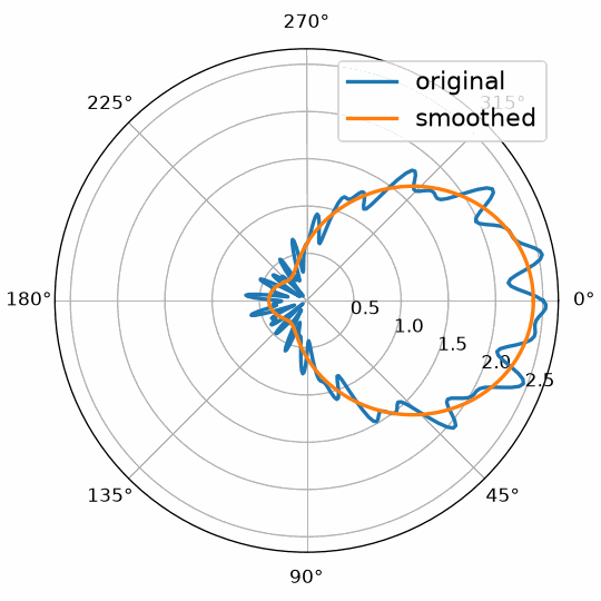
Read the smoothing result

The original curve has fine ripples from modes 20 and 35. The smoothed curve suppresses those ripples while retaining the broad mode-one and mode-two variation. Smoothing changes the function, so the halfwidth should be reported with any derived peak direction or density.

Compute integrals and extrema

Standard operations apply directly to an S1FunHarmonic. Here S1FH is still the bandwidth-20 approximation of \(\exp(\cos\rho)\). mean returns its mean value, while sum returns its integral over the circle.

meanValue = mean(S1FH)
meanValue

1.2661

integralValue = sum(S1FH)
integralValue

7.9549

max and min return both the extreme value and its angular position.

maxValue, maxPosition = max(S1FH)
minValue, minPosition = min(S1FH)
extremePositionsDegree = np.array([maxPosition, minPosition]) / degree
print(f'max {maxValue:.4f} at {extremePositionsDegree[0]:.1f}, min {minValue:.4f} at {extremePositionsDegree[1]:.1f}')

max 2.7183 at 0.0, min 0.3679 at 180.0

Read the operations

The mean is about 1.2661, and the integral is about 7.9549. Their ratio is \(2\pi\). The maximum is \(\mathrm e\) at zero degrees, while the minimum is \(\mathrm e^{-1}\) at 180 degrees.

Estimate a density from angular data

Periodic functions also arise after density estimation from circular data. For example, rho is the azimuth angle of a three-dimensional direction. Passing these angles with the periodic option makes calcDensity return an S1FunHarmonic.

v = vector3d.rand(1000, rng=np.random.default_rng(1))
fun = calcDensity(v.rho, periodic=True)
fun

S1FunHarmonic
  bandwidth: 60
  mean     : 1

densityMean = mean(fun)
densityMean

1.0000

plot(fun, lineWidth=2)

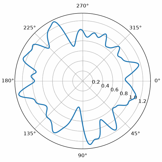
Read the angular density

The directions were sampled uniformly, so the density fluctuates around a flat value rather than forming a stable preferred direction. Its mean is one because calcDensity normalizes the periodic density. A pronounced reproducible peak would instead indicate a preferred azimuth.

The maths behind the Fourier representation

A \(2\pi\)-periodic function can be represented as a weighted sum of sines and cosines. MTEX uses the numerically convenient complex exponentials \(\mathrm e^{-\mathrm i k\rho}\). A finite series of bandwidth \(N\) is

MTEX uses the coefficient convention

The constant coefficient \(\hat f_0\) is therefore the mean value,

The integral returned by sum is

References

• H. Schaeben, The de la Vallee Poussin Standard Orientation Density Function, Textures and Microstructures 33 (1999), 365–373, relates the de la Vallee Poussin kernel to finite harmonic representations used for texture density estimation.

Next

Continue with Ellipse Based Shape Parameters to apply periodic density functions to grain long-axis and shortest-caliper directions.

Technical Details

MATLAB’s subplot(1,2,1) becomes a polar axes when a polar plot goes into it; with matplotlib the page asks for projection='polar'. The random directions are seeded by NumPy’s generator, not MATLAB’s rng default, so the density differs from MATLAB’s in its fluctuations.

@article{bachmann2010mtex,
  author  = {F. Bachmann and R. Hielscher and H. Schaeben},
  title   = {Texture Analysis with MTEX - Free and Open Source Software Toolbox},
  journal = {Solid State Phenomena},
  volume  = {160},
  pages   = {63-68},
  year    = {2010},
  doi     = {10.4028/www.scientific.net/SSP.160.63},
  url     = {https://doi.org/10.4028/www.scientific.net/SSP.160.63}
}