
MTEX for Python keeps the names of MATLAB MTEX: the classes (vector3d, orientation,
EBSD, grain2d), the commands (calcGrains, calcDensity, plotPF) and their
options. A MATLAB script translates line by line, and most lines change only in their
punctuation. This page lists what does change, the rules of the Python language first and
then the few places where MTEX itself behaves differently.
At a glance
| MATLAB | Python | |
|---|---|---|
| Start MTEX | startup_mtex, once per session |
from mtex import *, in every script |
| Editor | the MATLAB desktop | VS Code with the Python and Jupyter extensions |
| Section of a script | %%, run with Ctrl+Enter |
# %%, run with Shift+Enter |
| Comment | % text |
# text |
| Suppress output | ; at the end of a line |
not needed, only the last line of a cell prints |
| Option with a value | calcGrains(ebsd, 'angle', 10*degree) |
calcGrains(ebsd, angle=10*degree) |
| Flag | 'antipodal' |
antipodal=True |
| Select | ebsd('indexed') |
ebsd['indexed'] |
| First and last element | x(1), x(end) |
x[0], x[-1] |
| Several outputs | [grains, ebsd] = calcGrains(ebsd) |
grains = calcGrains(ebsd) |
| Copy | ori2 = ori |
ori2 = ori.copy() |
| Join | [ori1, ori2] |
cat(ori1, ori2) |
| Element-wise arithmetic | a .* b, a .^ 2 |
a * b, a ** 2 |
| Overlay plots | hold on |
hold(True) |
| Import wizard | import_wizard |
importWizard() |
| Open a documentation page | edit EBSDTutorial |
openDoc('EBSDTutorial') |
The sections below explain each row.
Starting MTEX
MATLAB MTEX is started once per session with startup_mtex. In Python, every script
starts by importing MTEX:
from mtex import *
This makes every MTEX command available by its name. The setup of Python and of an editor is described in Installing MTEX for Python.
Comments start with # instead of %, and a cell of the editor starts with # %%
instead of %%. There is no semicolon to suppress output: a line never prints anything,
except the last line of a cell when it is a bare expression. Use print to show a value
anywhere else.
ebsd = mtexdata('forsterite')
print(len(ebsd))
ebsd
245952
EBSD (y↓→x)
  size: 336 × 732 grid
  Phase  Orientations  Mineral     Color         Symmetry  Crystal reference frame
  0      58485 (24%)   notIndexed
  1      152345 (62%)  Forsterite  LightSkyBlue  mmm       Forsterite
  2      26058 (11%)   Enstatite   DarkSeaGreen  mmm       Enstatite
  3      9064 (3.7%)   Diopside    Goldenrod     12/m1     Diopside
  properties    : bands, bc, bs, error, mad
  scan unit     : um
  X × Y         : [0 → 3.655e+04] × [0 → 1.675e+04]
  square lattice: spacing 50
Options are keywords
A MATLAB option is a name followed by its value, a flag is a name alone. In Python both
are keyword arguments: the option is name=value, the flag is name=True.
| MATLAB | Python |
|---|---|
calcGrains(ebsd, 'angle', 10*degree) |
calcGrains(ebsd, angle=10*degree) |
Miller(1,0,0, cs, 'antipodal') |
Miller(1, 0, 0, cs, antipodal=True) |
plot(grains, 'linewidth', 2) |
plot(grains, lineWidth=2) |
calcODF(pf, 'noGhostCorrection') |
calcODF(pf, ghostCorrection=False) |
The keywords are spelled one way throughout: in camelCase (lineWidth, markerSize,
displayName), a tolerance as tol, an iteration bound as maxIter, and a flag by what
it switches on, so that MATLAB’s 'noSymmetry' is symmetry=False. Progress output is
switched by verbose, where MATLAB silences it by 'silent': mtexdata(..., verbose=False).
A string that names something stays a string in the argument list: the kind of Miller
indices 'uvw', an Euler convention 'ZYZ', an alignment 'X||a'.
grains = calcGrains(ebsd, angle=10 * degree, minPixel=5)
cs = ebsd['Forsterite'].CS
Miller(1, 0, 0, cs, 'uvw')
vector3d (Forsterite)
  u  v  w
  1  0  0
See Options for more.
Indexing with brackets, counting from zero
Selections use square brackets instead of round ones. Everything else about them stays: a phase name, a condition or a list of positions selects.
| MATLAB | Python |
|---|---|
ebsd('indexed') |
ebsd['indexed'] |
ebsd('Forsterite') |
ebsd['Forsterite'] |
grains(grains.grainSize > 100) |
grains[grains.grainSize > 100] |
gB('Forsterite', 'Forsterite') |
gB['Forsterite', 'Forsterite'] |
Positions count from 0, and a range a:b stops before b. MATLAB’s x(1) is x[0],
x(1:10) is x[0:10], and x(end) is x[-1].
big = grains[grains.grainSize > 100]
big[0:3].grainSize
array([2550, 427, 121], dtype=int32)
Positions and ids are different things: the grain ids count from 1, as in MATLAB, so the first grain is at position 0 and has the id 1.
grains[0].id
array([1], dtype=int32)
See Lists and Indexing for the details.
Properties and methods
What MATLAB MTEX calls a property is written without parentheses, a command with them.
MATLAB accepts rot.angle for angle(rot); Python needs the parentheses, and without them
returns the command itself instead of its result.
ori = ebsd['Forsterite'].orientations[0:3]
ori.CS
crystalFrame (⊙c→a)
  mineral : Forsterite
  symmetry: mmm
  elements: 8
  a, b, c : 4.756, 10.21, 5.98
ori.angle() / degree
array([50.9455, 50.9184, 51.0415])
Every such command is also a function, as in MATLAB: angle(ori) is ori.angle().
Several outputs
A command with several outputs returns them together, and they are unpacked by commas
instead of square brackets: MATLAB’s [ind, d] = find(...) is ind, d = find(...).
calcGrains is the exception. MATLAB also returns the updated map,
[grains, ebsd] = calcGrains(ebsd). Python writes the grain ids into the input map,
so grains = calcGrains(ebsd) suffices:
grains = calcGrains(ebsd, angle=10 * degree, minPixel=5)
ebsd.grainId[0:5]
array([[ 1,  1,  1, ..., 47, 47, 47],
       [ 1,  1,  1, ..., 47, 47, 47],
       [ 1,  1,  1, ...,  0, 47, 47],
       [ 1,  1,  1, ..., 46,  0,  0],
       [ 1,  1,  1, ...,  0, 58,  0]], dtype=int32)
Because the map is changed, compare two reconstructions on copies:
calcGrains(ebsd.copy(), ...).
Assignment does not copy
In MATLAB, ori2 = ori makes a copy, and changing ori2 leaves ori alone. In Python both
names refer to the same object, so a change through one is seen through the other. Ask for
a copy when you want one:
ori2 = ori.copy()
Operations never change their input: ori2 = ori * rot or ebsd2 = rotate(ebsd, rot)
return new objects, as in MATLAB.
Lists of objects
Square brackets in MATLAB concatenate: [ori1, ori2]. In Python square brackets build a
plain Python list, which MTEX commands do not accept as a list of orientations. Use cat:
ori1 = orientation.byEuler(0, 0, 0, cs)
ori2 = orientation.byEuler(90 * degree, 0, 0, cs)
cat(ori1, ori2)
orientation (Forsterite → y↓→x)
  size: 2
  Bunge Euler angles in degree
  phi1  Phi  phi2
     0    0     0
    90    0     0
Arithmetic, numbers and control flow
The operations on MTEX objects keep their meaning: * applies a rotation, inv(ori)
inverts. For numbers, MTEX uses NumPy, the standard Python package for arrays, whose
operations apply elementwise without a dot.
| MATLAB | Python |
|---|---|
a .* b, a ./ b, a .^ 2 |
a * b, a / b, a ** 2 |
a ~= b, ~a |
a != b, ~a |
a && b, a \|\| b |
a and b, a or b |
zeros(3, 1), mean(x), max(x) |
np.zeros(3), np.mean(x), np.max(x) |
numel(x) |
len(x) or x.size |
isnan(x) |
np.isnan(x) |
pi, degree |
pi, degree |
for i = 1:n ... end |
for i in range(n): and an indented block |
if a > 0 ... end |
if a > 0: and an indented block |
function y = f(x) ... end |
def f(x): and an indented block ending in return y |
sprintf('%d grains', n) |
f'{n} grains' |
Python has no end: the lines of a loop or a function are the ones indented below it.
NumPy is imported as import numpy as np.
import numpy as np
for i in range(3):
  print(f"grain {big[i].id[0]}: {big[i].grainSize[0]} pixels")
grain 1: 2550 pixels
grain 4: 427 pixels
grain 7: 121 pixels
Plotting
The plotting commands are MATLAB MTEX’s and take the same options. Figures are drawn with matplotlib, the standard plotting package of Python.
| MATLAB | Python |
|---|---|
figure |
newMtexFigure() |
hold on, hold off |
hold(True), hold(False) |
nextAxis |
nextAxis() |
mtexColorbar |
mtexColorbar() |
saveFigure('map.png') |
saveFigure('map.png') |
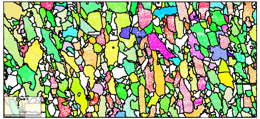
plot(ebsd['Forsterite'], ebsd['Forsterite'].orientations)
hold(True)
plot(grains.boundary, lineWidth=1.5)
hold(False)
Names that changed
A few classes carry the names of the coming MATLAB release, where the MATLAB pages of MTEX 6 still use the old ones, and a few commands have a better name in Python than in MATLAB: a misnomer, a duplicate or a workaround for a limit of MATLAB. They take the same arguments.
| MATLAB MTEX 6 | Python |
|---|---|
crystalSymmetry('m-3m', [a b c], 'mineral', 'Iron') |
crystalFrame('m-3m', [a, b, c], mineral='Iron') |
specimenSymmetry('222') |
specimenFrame('222') |
ebsd.opt |
ebsd.meta |
loadEBSD(fname) |
loadEBSD(fname) or EBSD.load(fname) |
import_wizard |
importWizard(), or mtex-wizard in a terminal |
plotPDF(odf, h), plotPDF(ori, h) |
plotPF(odf, h), plotPF(ori, h) |
plotIPDF(odf, r), plotIPDF(ori, r) |
plotIPF(odf, r), plotIPF(ori, r) |
calcPDF(odf, h, r), odf.pdf(h) |
odf.radon(h, r), odf.radon(h) |
odf.ipdf(r) |
odf.radon(r=r) |
hist(grains) |
histogram(grains, grouped=True) |
angle_outer(v1, v2), dot_outer(v1, v2) |
angle(v1, v2, outer=True), dot(v1, v2, outer=True) |
eq(v1, v2), eqTol(cs1, cs2) |
isclose(v1, v2), isclose(cs1, cs2) |
orientation.eye(cs) |
orientation.id(cs) |
plotSpektra(odf) |
plotSpectrum(odf) |
textureindex(odf) |
textureIndex(odf) |
eS.addFeature_singleStep |
eS.addFeature('singleStep') |
project2FundamentalRegion(ori) |
projectIntoFundamentalRegion(ori) |
project2EulerFR(ori) |
projectIntoEulerRegion(ori) |
sR.restrict2Upper |
sR.restrictToUpper |
SO3F.SRight, SO3F.SLeft, oR.CS1, oR.CS2 |
SO3F.frameA, SO3F.frameB (or CS, SS) |
plotx2north |
plottingConvention.default(north=xvector) |
quiver3(t) |
quiver3d(t) |
loadEBSD_ang(fname) |
loadEBSD(fname), the format from the extension or interface='ang' |
export_VPSC(ori, fname) |
export(ori, fname, interface='VPSC') |
Behaviour that differs on purpose
==compares coordinates.v1 == v2of vectors, rotations, orientations, fibres or tangent vectors is true where the coordinates are equal (for rotations up to the sign of the quaternion); MATLAB’s==compares within a tolerance and up to symmetry, which isisclose(v1, v2)orv1.isclose(v2, tol=...)here.calcGrainschanges the map it is given, as described above.- A map read on a grid keeps its grid. A map whose file stores a regular grid is a
two-dimensional EBSD object at once, rows by columns, where MATLAB reads a list and
builds the grid by
gridify. A selection such asebsd['indexed']is a list. - Moving a gridded map keeps the order of its data.
rotate,shiftandtransformmove the positions; MATLAB stores a rotated map anew.gridify(ebsd, ...)reorders explicitly. - Unknown options.
calcGrainsand most computing commands refuse a misspelt keyword; the plotting commands pass unknown ones on to matplotlib.
print(ebsd.shape, ebsd['indexed'].shape)
(336, 732) (226906,)
Where to find help
Every page of the MTEX documentation has a MATLAB and a Python version; the switch at the
top of a page changes between them. The MATLAB page is the place to look for anything
this port does not describe yet, and the rules of this page translate its code.
openDoc('EBSDTutorial') gives a page as a script to run section by section, as
edit EBSDTutorial opens a documentation script in MATLAB.
The Python Tutorial is the introduction to the
language, NumPy for MATLAB users
the translation table for numerical code.
Citing this page.
This page is part of the documentation of
MTEX, a free and open
source MATLAB toolbox for analyzing and modeling crystallographic textures.
It was written by The MTEX Developers and is published at
https://mtex-toolbox.github.io/MATLABtoPython_py.html.
If you use MTEX, or reuse text or figures from this page, in your research,
please cite
F. Bachmann, R. Hielscher, H. Schaeben: Texture Analysis with MTEX - Free and Open Source Software Toolbox, Solid State Phenomena 160 (2010), 63-68. 10.4028/www.scientific.net/SSP.160.63
BibTeX
@article{bachmann2010mtex,
  author  = {F. Bachmann and R. Hielscher and H. Schaeben},
  title   = {Texture Analysis with MTEX - Free and Open Source Software Toolbox},
  journal = {Solid State Phenomena},
  volume  = {160},
  pages   = {63-68},
  year    = {2010},
  doi     = {10.4028/www.scientific.net/SSP.160.63},
  url     = {https://doi.org/10.4028/www.scientific.net/SSP.160.63}
}
Other papers describing specific MTEX methods are listed under Publications — please cite the one that best fits your application. The MTEX source code is licensed under the GNU General Public License v2.0; the text and figures of this documentation are licensed under CC BY 4.0, which permits reuse — including by automated systems — provided The MTEX Developers and this page are credited.