Operations on Crystal Directions and Planes

A Miller represents either a direct-lattice vector \([uvw]\) or a reciprocal-lattice normal \((hkl)\) in a crystal frame. It supports ordinary vector geometry, but comparisons have one extra input: crystal symmetry.

By default, angle, dot and eq compare a vector with the symmetry orbit of the other vector. In contrast, constructions such as cross act on the indexed vectors actually supplied. This page shows when to keep the default and when to request symmetry=False.

Read Miller Indices and Lattice Metric and Plane Geometry first if direct and reciprocal indices are new. Crystal Symmetries introduces the point groups used here, while Axes and Antipodal Symmetry explains when opposite vectors represent the same axis.

import matplotlib.pyplot as plt
import numpy as np

from mtex import *

plottingConvention.default('y↑→x')

A Kikuchi Pattern as a Geometric Map

A simulated spherical Kikuchi pattern of quartz makes the operations visible. This is a master pattern on the sphere, not a raw planar detector image. The left plot shows the pattern, and the right plot shows its spherical Radon transform.

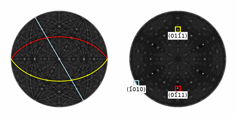
A band centre is a great circle on the pattern. The transform maps that great circle to the point representing its plane normal.

pattern = mtexdata('quartzPattern')

plot(pattern, resolution=0.25 * degree, complete=True, upper=True, axisLabels=False)
mtexColorMap('black2white')
ax1 = gcm().children[-1]
nextAxis()
plot(pattern.radon(), resolution=0.25 * degree, complete=True, upper=True, axisLabels=False)
mtexColorMap('black2white')
ax2 = gcm().children[-1]

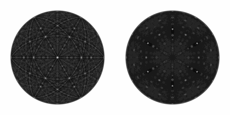
The brightest bands belong to three strongly reflecting quartz forms: the hexagonal prism and the positive and negative rhombohedra. Each form is introduced below by one plane normal.

# extract the crystal symmetry
cs = pattern.CS

m = Miller(-1, 0, 1, 0, cs, 'hkil')  # hexagonal prism
r = Miller(0, -1, 1, 1, cs, 'hkil')  # positive rhombohedron
z = Miller(0, 1, -1, 1, cs, 'hkil')  # negative rhombohedron

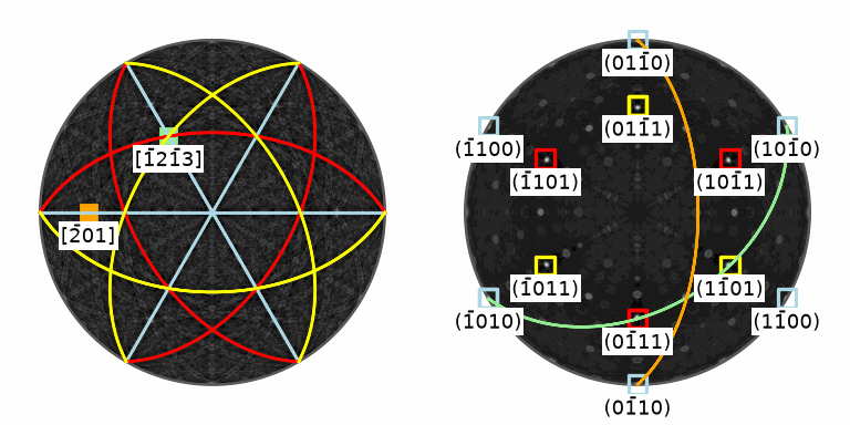
Drawn in both plots, a plane is a great circle on the left and a point on the right. The matching colours identify the same plane in the two representations.

hold(True)
circle(m, parent=ax1, color='lightBlue')
circle(r, parent=ax1, color='red')
circle(z, parent=ax1, color='yellow')

opt = dict(marker='s', markerFaceColor='none', parent=ax2, labeled=True, backgroundColor='w', lineWidth=2)
plot(m, **opt, markerEdgeColor='lightBlue')
plot(r, **opt, markerEdgeColor='red')
plot(z, **opt, markerEdgeColor='yellow')

Symmetrically Equivalent Planes and Directions

A symmetry orbit contains the vectors obtained by applying every operation of the crystal point group. Its members are symmetrically equivalent because the crystal cannot distinguish the corresponding settings.

The family of directions equivalent to \([uvw]\) is written \(\langle uvw\rangle\). The family of planes equivalent to \((hkl)\) is written \(\{hkl\}\). symmetrise lists the orbit as directed vectors.

symmetrise(r)

vector3d (Quartz)
  size: 6
   h   k   i   l
   0  -1   1   1
   1   0  -1   1
   0   1  -1  -1
  -1   1   0   1
  -1   0   1  -1
   1  -1   0  -1

Quartz point group 321 has six operations, and none repeats this normal. The output therefore contains six directed normals. For this rhombohedron they form three opposite pairs.

A geometric plane is unchanged when its normal is reversed. Thus the six directed normals describe three distinct plane axes. Adding the symmetry orbits to the plots accounts for the corresponding bands.

hold(True)
circle(m.symmetrise(), parent=ax1, color='lightBlue')
circle(r.symmetrise(), parent=ax1, color='red')
circle(z.symmetrise(), parent=ax1, color='yellow')

plot(m, **opt, markerEdgeColor='lightBlue', symmetrised=True)
plot(r, **opt, markerEdgeColor='red', symmetrised=True)
plot(z, **opt, markerEdgeColor='yellow', symmetrised=True)

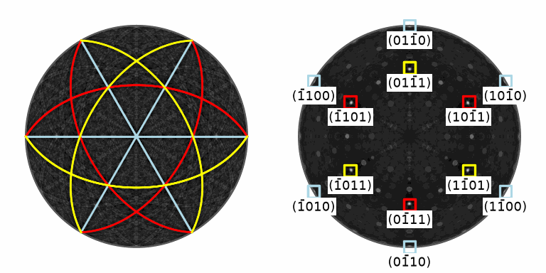
The option symmetrised on plot performs the same expansion. A plain symmetrise call keeps one entry per symmetry operation and may contain repeated vectors. Use unique when the number of distinct members is the question.

directedNormalCount = len(symmetrise(r, unique=True, antipodal=False))
directedNormalCount

6

The first count keeps opposite normals distinct. The antipodal option instead treats a vector and its negative as the same axis.

planeAxisCount = len(symmetrise(r, unique=True, antipodal=True))
planeAxisCount

3

The two outputs are 6 directed normals and 3 plane axes. Point-group equivalence and antipodal equivalence are separate choices; select the one that matches the physical object being described.

Multiplicity

The multiplicity is the number of distinct directed vectors in a symmetry orbit. It is the count returned by symmetrise(..., unique=True, antipodal=False). A direction on a symmetry axis has lower multiplicity because some operations leave it fixed.

For diffraction with Friedel equivalence, opposite reflection normals contribute together. Using a Laue group includes that equivalence in the conventional multiplicity factor for a powder reflection.

csCubic = crystalFrame('m-3m')
hCubic = Miller([[1, 0, 0], [1, 1, 0], [1, 1, 1]], csCubic)

multiplicity(hCubic)

array([ 6, 12,  8])

The cubic \(\{100\}\), \(\{110\}\) and \(\{111\}\) forms have multiplicities 6, 12 and 8. The order of the indices does not determine this count; the stabilising symmetry of the direction does.

Are Two Normals Equivalent?

The two objects below are opposite directed normals. The operator == asks whether point group 321 maps one normal onto the other.

r1 = Miller(1, 1, -2, 0, cs, 'hkil')
r2 = Miller(-1, -1, 2, 0, cs, 'hkil')

r1 == r2

False

The result is false because no operation of 321 makes that mapping. Treating the normals as axes makes their signs irrelevant.

isclose(r1, r2, antipodal=True)

True

The second result is true. This distinction matters whenever directed crystal vectors, plane axes and Friedel-equivalent reflections appear in the same calculation.

Does a Direction Lie in a Plane?

A direction \([uvw]\) lies in a plane \((hkl)\) when their scalar product is zero. In three-index notation this is the zone law

Incidence concerns the two indices that were written. Use symmetry=False so that dot does not substitute a symmetry-equivalent vector.

csOrtho = crystalFrame('mmm', [4, 5, 6])
plane = Miller(1, 1, 0, csOrtho, 'hkl')
directionInPlane = Miller(1, -1, 0, csOrtho, 'uvw')

dot(plane, directionInPlane, symmetry=False)

0

Zero confirms that \([1\bar{1}0]\) lies in \((110)\). In contrast, the result for \([100]\) is 1, so that direction does not lie in the plane.

dot(plane, Miller(1, 0, 0, csOrtho, 'uvw'), symmetry=False)

1

This Cartesian dot-product test also works with four-index trigonal and hexagonal notation. There is no need to translate the indices manually.

Zone Axes and Spanned Planes

Two lattice planes intersect along a lattice direction called a zone axis. Its direction is the cross product of their reciprocal normals.

d1 = round(cross(m, r))
d1

vector3d (Quartz)
   U  V   T  W
  -1  2  -1  3

plot(d1, marker='s', parent=ax1, markerFaceColor='lightgreen', labeled=True, backgroundColor='w')
circle(d1, parent=ax2, lineColor='lightgreen')

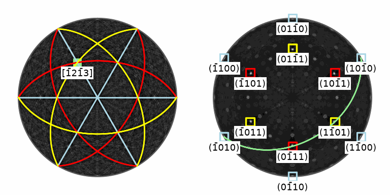
The output uses UVTW because a cross product of two reciprocal normals is a direct-lattice direction. round rescales it to small integer indices.

The green square lies where the two corresponding bands cross in the pattern. In the Radon plot, its green great circle passes through their two normal points.

d2 = Miller(-2, 0, 1, cs, 'uvw')
d2

vector3d (Quartz)
   u  v  w
  -2  0  1

plot(d2, marker='s', parent=ax1, markerFaceColor='orange', labeled=True, backgroundColor='w')
circle(d2, parent=ax2, lineColor='orange')

Conversely, two direct-lattice directions span a plane. Their cross product is displayed in reciprocal hkil notation.

n = round(cross(d1, d2))
n

vector3d (Quartz)
  h   k  i  l
  1  -2  1  2

circle(n, parent=ax1, lineColor='white')
plot(n, **opt, markerEdgeColor='white')

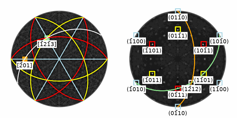
The white band contains d1 and d2 in the pattern. In the Radon plot, the white normal lies where the green and orange great circles intersect.

Symmetry-Reduced and Geometric Angles

By default, angle returns the smallest angle between the first vector and the symmetry orbit of the second. The result is independent of which equivalent index triplet was supplied.

symmetryAngle = angle(r1, r2) / degree
symmetryAngle

60.0000

The point-group-reduced angle is \(60^\circ\). If the normals represent plane axes, include antipodal equivalence as well.

axisAngle = angle(r1, r2, antipodal=True) / degree
axisAngle

0

The result is numerically close to zero. To compare only the two Cartesian vectors as written, ignore crystal symmetry.

geometricAngle = angle(r1, r2, symmetry=False) / degree
geometricAngle

180

The geometric angle is \(180^\circ\) because the normals are exactly opposite. Thus the same two index sets give a \(60^\circ\) point-group angle, a near-zero plane-axis angle and a \(180^\circ\) geometric angle.

The option symmetry=False is available to many commands that accept crystal directions or orientations. Use it when the indexed vectors themselves, rather than their symmetry classes, are the subject.

From the Crystal Frame into the Specimen Frame

An orientation states how a crystal is placed in the specimen. It maps a direction from the Cartesian crystal frame into the specimen frame.

ori = orientation.byEuler(10 * degree, 20 * degree, 30 * degree, 'Bunge', cs)

plt.close('all')
plot(ori * pattern, resolution=0.25 * degree, complete=True, upper=True)
mtexColorMap('black2white')

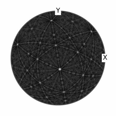
The whole pattern has moved rigidly with the crystal. Multiplying the zone axis by the same orientation returns a specimen direction rather than a Miller object.

specimenDirection = ori * d1
specimenDirection

vector3d (y↑→x)
      x       y     z
  -4.27  -0.286  5.92

hold(True)
plot(specimenDirection, marker='s', markerFaceColor='lightgreen', label=d1.char(family=False), backgroundColor='w')
hold(False)

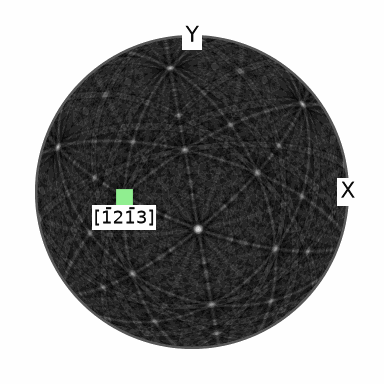
Applying the orientation to the full symmetry orbit marks every specimen direction in which this crystal family points.

hold(True)
plot(ori * d1.symmetrise(), marker='s', markerFaceColor='lightgreen', label=d1.char(family=False), backgroundColor='w')
hold(False)

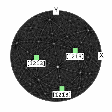
That set is the pole figure of this one orientation for the family represented by d1.

Cartesian Components Without Crystal Metadata

Building a vector3d from the Cartesian components of a Miller drops the crystal symmetry and crystal frame. The result is frame-free: it has an empty frame and resolves against the session default when it is rendered.

cartesianDirection = vector3d(d1.x, d1.y, d1.z)
cartesianDirection

vector3d (y↑→x)
      x     y     z
  -2.46  4.26  5.41

The frame name shown in the display is therefore the current session default, not a frame stored by the vector. The empty stored frame confirms that distinction.

isFrameFree = cartesianDirection.frame is None
isFrameFree

True

The result is true. This cast is not a frame change; it removes the information needed to interpret the components as lattice indices. A true frame change re-expresses the same physical object in a named frame and leaves the object itself untouched.

The ordinary spherical coordinates remain available: the polar angle from +Z and the azimuth from +X, in degrees.

np.array([d1.theta, d1.rho]) / degree

array([ 42.2705, 120.    ])

References

• The International Union of Crystallography, Zone axis, defines the zone axis and the Weiss zone law used for the incidence test.
• U. Shmueli, Reciprocal space in crystallography, International Tables for Crystallography B, ch. 1.1, 2006, develops the direct and reciprocal geometry behind these operations.
• A. Looijenga-Vos and M. J. Buerger, Space-group determination and diffraction symbols, International Tables for Crystallography A, ch. 3.1, 2006, explains Friedel equivalence and Laue symmetry in diffraction.
• N. C. Krieger Lassen, D. Juul Jensen and K. Conradsen, Image Processing Procedures for Analysis of Electron Back Scattering Patterns, Scanning Microscopy 6, article 7, 1992, introduces transform-based localisation of Kikuchi bands for automated indexing.
• A. Morawiec, Orientations and Rotations: Computations in Crystallographic Textures, Springer, 2004, develops symmetry orbits and symmetry-reduced angles for texture analysis.

Next

Continue in chapter order with Reference System, which explains how the lattice basis is embedded in the Cartesian crystal frame. Fundamental Sector later selects one representative from each symmetry-equivalent direction family.

Continue with Defining Orientations to place a crystal in a specimen. Pole Figures then plots where selected crystal directions point in that specimen.

Technical Details

The quartz master pattern is MATLAB’s quartzPattern.mat, a v7.3 object file; the sample data set quartzPattern reads its harmonic coefficients with h5py into the frame they are written in, point group 321 with the a axis along x. vector3d(m) keeps the crystal frame here, the frame-free vector is built from the components. MATLAB’s polar(d1) without an output prints the two angles in degrees; here they are the properties theta and rho.

@article{bachmann2010mtex,
  author  = {F. Bachmann and R. Hielscher and H. Schaeben},
  title   = {Texture Analysis with MTEX - Free and Open Source Software Toolbox},
  journal = {Solid State Phenomena},
  volume  = {160},
  pages   = {63-68},
  year    = {2010},
  doi     = {10.4028/www.scientific.net/SSP.160.63},
  url     = {https://doi.org/10.4028/www.scientific.net/SSP.160.63}
}