Boundary Plots

A grain boundary is stored as short segments between neighboring EBSD pixels that belong to different grains. A value attached to each segment can therefore be drawn as the colour of that short line.

The right colour encoding depends on the value. A misorientation angle is one number and needs a colorbar. A misorientation axis is a direction and needs a direction key. The full misorientation has three parameters and needs a key for rotation space.

This page assumes that the map has already been divided into grains. See Select Grain Boundaries for choosing segments and Theory of Misorientations for the angle-axis description used below.

import numpy as np
from mtex import *

# import the data in its specimen reference frame
plottingConvention.default('y↑→x')
ebsd = mtexdata('forsterite')

# restrict the map to a subregion of interest
ebsd = ebsd[inpolygon(ebsd, np.array([5, 2, 10, 5]) * 1000)]

# reconstruct grains with an explicit 15 degree threshold
grains = calcGrains(ebsd, angle=15 * degree, minPixel=5, alpha=10)

# ebsdId is used below, so keep each segment tied to its measured pixel pair
grains = smoothBoundary(grains, 4, simplify=False, refine=False)

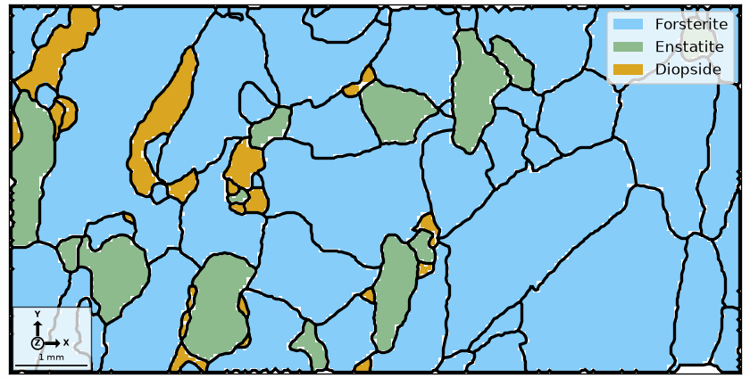
One colour for every boundary

With no data argument, plot draws all boundary segments in one colour on top of the phase map.

gB = grains.boundary

plot(ebsd)
hold(True)
plot(gB, lineWidth=2)
hold(False)

The misorientation angle

The misorientation angle is the smallest rotation angle relating the two crystal orientations. It is a useful first separation between low-angle boundaries within deformed grains and high-angle boundaries between grains.

gB_Fo = grains.boundary['Fo', 'Fo']

plot(grains, translucent=1, micronbar='off')
legend('off')
hold(True)
plot(gB_Fo, gB_Fo.misorientation.angle() / degree, lineWidth=4)
hold(False)
mtexColorbar(title='misorientation angle (°)')

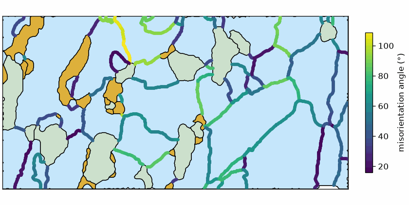
The colour is nearly constant along each boundary and changes between neighboring grains. The angles run from 15.9 to 108.8 degrees, with a median of 56.4 degrees.

Nothing below 15 degrees can appear because grain reconstruction used that threshold. Every segment in gB_Fo is therefore a high-angle boundary by construction. Subgrain Boundaries shows how to retain and plot the low-angle boundaries inside grains.

The misorientation axis in crystal coordinates

The axis is a direction, so a colorbar would be meaningless. Expressed in crystal coordinates, it identifies lattice directions about which the neighboring crystals are rotated.

Crystal symmetry gives several equivalent descriptions of the same axis. HSVDirectionKey folds them into one fundamental sector and assigns one colour to each direction there.

# axes in the forsterite crystal frame
axesCrystal = gB_Fo.misorientation.axis()

# construct the key and convert each axis to RGB
axisKey = HSVDirectionKey(axesCrystal)
axisColor = axisKey.direction2color(axesCrystal)

plot(grains, translucent=1, micronbar='off')
legend('off')
hold(True)
plot(gB_Fo, lineColor='black', lineWidth=6)
plot(gB_Fo, axisColor, lineWidth=4)
hold(False)

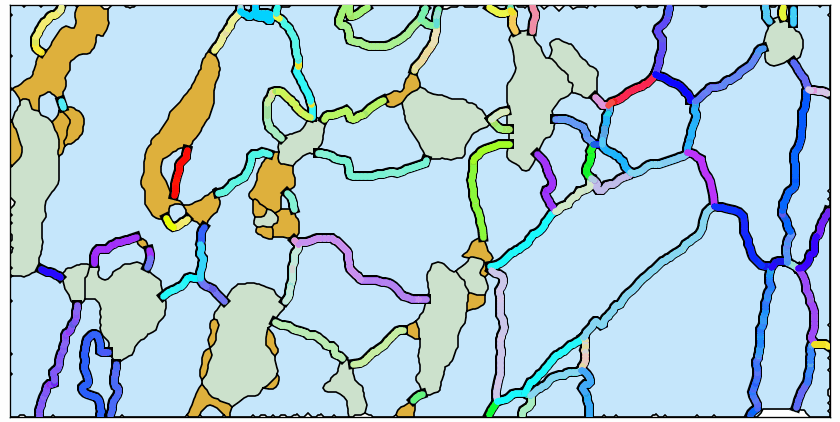
The black underlay keeps pale colours visible against the map. Read each boundary colour from the direction key below, not from a numerical colorbar.

plot(axisKey)
hold(True)
plot(axesCrystal, markerFaceAlpha=0.1, markerEdgeAlpha=0.3, markerFaceColor='black')
hold(False)

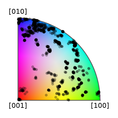
The black points show which part of the key the measured axes use. Their clusters reveal preferred crystal directions that are difficult to see from the coloured boundary map alone.

The misorientation axis in specimen coordinates

The same axis can be expressed in the specimen reference frame. It then describes how the two lattices are related in space rather than which crystal direction is involved.

The misorientation stored on a segment is a crystal-to-crystal rotation, so it no longer contains the specimen frame. The two measured orientations on either side are needed, and ebsdId leads back to them.

plot(grains, translucent=1, micronbar='off')
legend('off')
hold(True)
plot(gB_Fo, axisColor, lineWidth=4)

# boundary segments are in walk order, so sample every fifth one
gB_sample = gB_Fo[::5]

# retrieve the two measured orientations beside each sampled segment
ori = ebsd['id', gB_sample.ebsdId].orientations

# compute the same axes in the specimen reference frame
axesSpecimen = axis(ori[:, 0], ori[:, 1], antipodal=True)

quiver(gB_sample, axesSpecimen, autoScaleFactor=0.4, color='black')
hold(False)

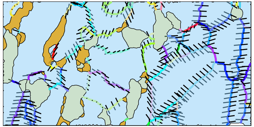
Sampling every fifth segment keeps the arrows readable without changing the boundary map. Because segments are stored in walk order, the arrows remain distributed along the boundary chains.

Each line is the projection of an axis into the measurement surface. A short line is therefore not a small rotation. It is an axis pointing steeply out of the section plane.

Symmetry reduction can also make neighboring segments choose different equivalent axes, especially near the largest possible misorientation angle. Misorientations at Grain Boundaries explains how to recognize that jump.

Colouring the whole misorientation

Angle and axis together are three parameters. The PatalaColorKey maps all three to a single RGB colour using the construction of S. Patala, J. K. Mason and C. A. Schuh, Improved representations of misorientation information for grain boundary science and engineering, Prog. Mater. Sci. 57, 1383-1425, 2012.

The key includes grain-exchange symmetry: viewing a same-phase boundary from the other side gives the inverse misorientation but not a different boundary. Its implementation is available for the Laue groups m-3m, m-3, mmm, 4/mmm and 6/mmm.

plot(grains, micronbar='off')
legend('off')

foKey = PatalaColorKey(gB_Fo)
foColor = foKey.orientation2color(gB_Fo.misorientation)

hold(True)
plot(gB_Fo, lineColor='black', lineWidth=7)
plot(gB_Fo, foColor, lineWidth=4)
hold(False)

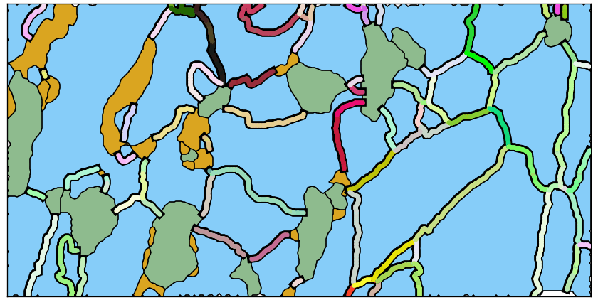
Two segments with the same colour now have the same misorientation, axis and angle alike, rather than merely the same angle. The black underlay again separates pale boundary colours from the phase map.

A three-parameter key cannot be displayed in one flat legend. MTEX shows axis angle sections, each at a fixed misorientation angle, and draws the measured misorientations on top.

plot(foKey, layout=[3, 4], figSize='large')
plot(gB_Fo.misorientation, markerFaceColor='none', add2all=True, markerSize=4)

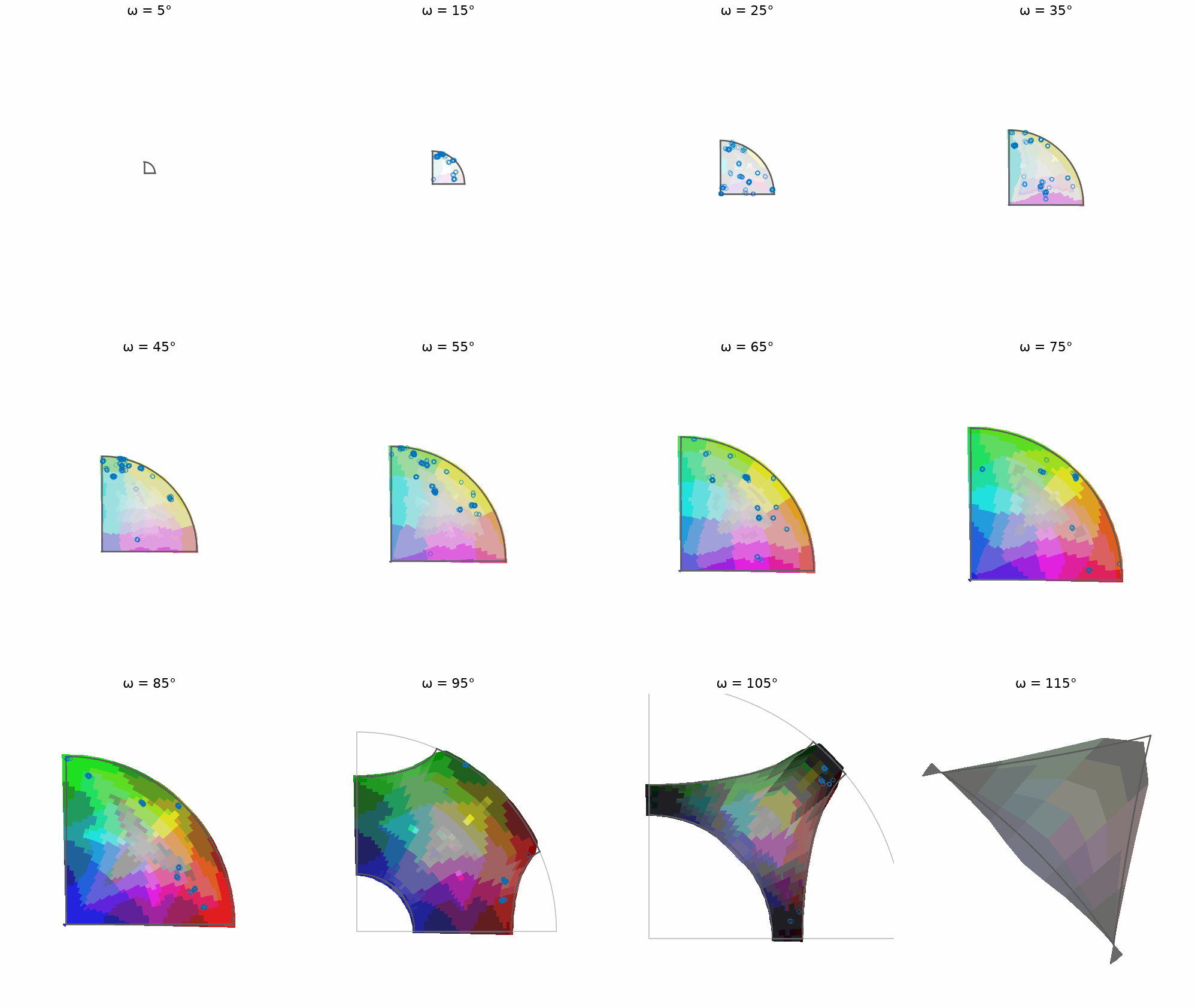
The forsterite misorientations fill the large-angle sections and leave the small-angle sections nearly empty. A preferred boundary relationship would instead appear as points gathered in one part of the key, with the corresponding colour repeated across the map.

A material with preferred boundary relationships

The iron sample below provides that comparison. Its plotting convention is reset explicitly because this specimen uses a different reference frame from the forsterite map.

plottingConvention.default('y↓→x')
ebsd = mtexdata('csl')

# reconstruct and smooth the grains
grains = calcGrains(ebsd)
grains = smoothBoundary(grains, 2)
gB = grains.boundary['iron', 'iron']

# plot image quality beneath a translucent orientation map
with np.errstate(divide='ignore'):
  logIq = np.log(ebsd.prop['iq'])
plot(ebsd, logIq, figSize='large', colormap='black2white', colorRange=[0.5, 5])

hold(True)
plot(grains, grains.meanOrientation, faceAlpha=0.4)

# colour the boundaries by their full misorientation
ironKey = PatalaColorKey(gB)
ironColor = ironKey.orientation2color(gB.misorientation)
plot(gB, ironColor, lineWidth=4)
hold(False)

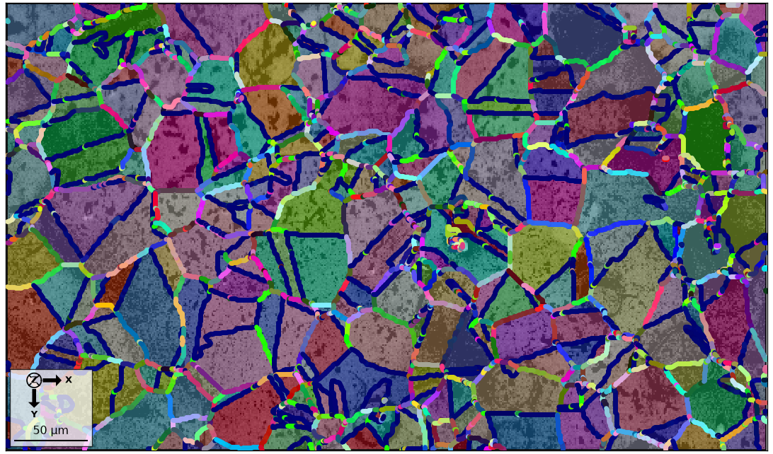
Whole boundaries now repeat one colour instead of changing continually along their length. Dark blue recurs across the map, so many boundaries share one misorientation. These are special boundaries, and CSL Boundaries identifies their relationships.

plot(ironKey, 'axisAngle', axisAngle=np.arange(5, 61, 5) * degree, layout=[4, 3], figSize='large')

moriSample = discreteSample(gB.misorientation, 300, withoutReplacement=True)

plot(moriSample, add2all=True, markerFaceColor='none', markerEdgeColor='w')

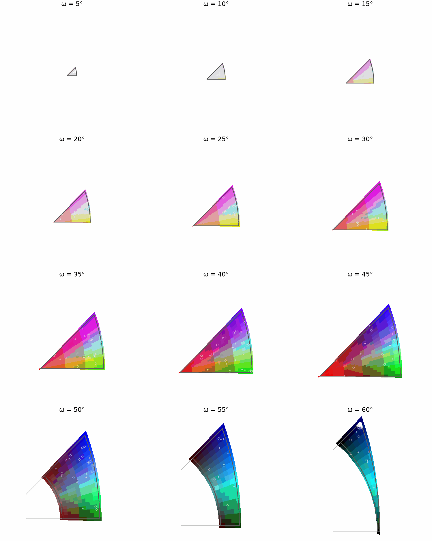
The sections confirm the clustering: 300 measured misorientations occupy a few small parts of the key instead of filling the available space. A misorientation and its inverse are drawn at the same place because they describe the same boundary viewed from opposite sides.

What the colours do not describe

The Patala colour contains the full three-parameter misorientation, not the full grain-boundary character. Two further parameters specify the boundary-plane orientation. A two-dimensional EBSD map measures only the plane trace and cannot recover its inclination from one boundary.

The same colour therefore does not by itself imply the same boundary energy, structure or chemistry. See Grain Boundaries for the five-parameter description and Boundary Normal Distribution for what can be inferred from many traces.

Further reading

• A. Morawiec, Orientations and Rotations: Computations in Crystallographic Textures, Springer, 2004, develops rotation space, crystal symmetry and misorientation axes.
• A. P. Sutton, E. P. Banks and A. R. Warwick, The five-dimensional parameter space of grain boundaries, Proc. R. Soc. A 471, 20150442, 2015, separates the three misorientation parameters from the two boundary-plane parameters.
• S. Patala, J. K. Mason and C. A. Schuh, Improved representations of misorientation information for grain boundary science and engineering, Prog. Mater. Sci. 57, 1383-1425, 2012, constructs the colour key used here for a complete misorientation.
• F. Bachmann, R. Hielscher and H. Schaeben, Grain detection from 2d and 3d EBSD data - Specification of the MTEX algorithm, Ultramicroscopy 111, 1720-1733, 2011, explains how EBSD measurements become grains and boundary segments.

Technical Details

ebsd['id', M] returns one measurement per entry of the matrix M, in its shape, so the two columns of ebsdId give the two orientation lists. axis(o1, o2) is their misorientation axis in the specimen frame. gB_Fo[::5] is MATLAB’s gB_Fo(1:5:end).

@article{bachmann2010mtex,
  author  = {F. Bachmann and R. Hielscher and H. Schaeben},
  title   = {Texture Analysis with MTEX - Free and Open Source Software Toolbox},
  journal = {Solid State Phenomena},
  volume  = {160},
  pages   = {63-68},
  year    = {2010},
  doi     = {10.4028/www.scientific.net/SSP.160.63},
  url     = {https://doi.org/10.4028/www.scientific.net/SSP.160.63}
}