
An anisotropic crystal has two permitted polarization directions for most light-propagation directions. The two waves travel at different speeds. Their refractive-index difference is the directional birefringence.
Between crossed polarizers, this speed difference becomes a phase lag. Some wavelengths are then transmitted more strongly than others, producing the interference colours seen in a petrographic microscope.
This page builds a rank-two refractive-index tensor for olivine. It then predicts birefringence, optical axes, and interference colours from EBSD orientations. The tensor and orientation conventions are introduced in Tensor Definition and Orientations. The distinction between crystal symmetry and its frame is explained in Crystal Reference Systems.
import numpy as np
from mtex import *
Load an orientation map
The olivine data uses transverse direction (TD) upward and rolling direction (RD) to the right. The explicit plotting convention states that specimen frame rather than inheriting the session default.
plottingConvention.default('y↑→x')
ebsd = mtexdata('olivine')

grains = calcGrains(ebsd, minPixel=5)
olivine = ebsd['olivine']

ipfKey = ipfColorKey(olivine)
ipfColors = ipfKey.orientation2color(olivine.orientations)

plot(olivine, ipfColors)
hold(True)
plot(grains.boundary, lineWidth=1.5)
hold(False)
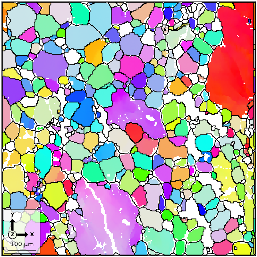
This inverse pole figure (IPF) map is the orientation reference for the optical maps below. Neighbouring grains have different colours because their crystal frames have different orientations in the specimen frame. These IPF colours do not represent an optical response.
Build the refractive-index tensor
The refractive index is \(n=c/v\), so a larger index means a slower wave. A symmetric rank-two tensor stores its directional dependence. refractiveIndexTensor attaches that tensor to the crystal frame.
Orthorhombic olivine is optically biaxial. Its three principal indices are \(n_{\alpha}<n_{\beta}<n_{\gamma}\), with \(n_{\alpha}\) parallel to b, \(n_{\beta}\) parallel to c, and \(n_{\gamma}\) parallel to a. The order in the diagonal matrix is therefore a, b, c.
The mmm point group forces the off-diagonal components to zero in this symmetry-aligned crystal frame. Symmetry constrains the property, while the frame states which axes its components refer to. MTEX carries both with the tensor.
cs = olivine.CS

nAlphaFo = 1.635
nBetaFo = 1.651
nGammaFo = 1.670
rIFo = refractiveIndexTensor(np.diag([nGammaFo, nAlphaFo, nBetaFo]), cs)

nAlphaFa = 1.827
nBetaFa = 1.869
nGammaFa = 1.879
rIFa = refractiveIndexTensor(np.diag([nGammaFa, nAlphaFa, nBetaFa]), cs)
An illustrative solid-solution model
Olivine forms a solid solution between forsterite and fayalite. For this example, the forsterite mole fraction is fixed at 0.86 and the two end-member tensors are interpolated linearly. This is a modelling assumption, not a composition inferred from the EBSD map.
xFo = 0.86
rI = xFo * rIFo + (1 - xFo) * rIFa

# rows: forsterite, fayalite, the Fo86 model, columns: n_a, n_b, n_c
principalIndices = np.array([np.diag(rIFo.M), np.diag(rIFa.M), np.diag(rI.M)])
principalIndices
array([[1.67  , 1.635 , 1.651 ],
       [1.879 , 1.827 , 1.869 ],
       [1.6993, 1.6619, 1.6815]])
The rows show why the axis assignment matters. Sorting the three values and placing them on a, b, c in that order would describe a different material. The tensor must also remain attached to the same crystal frame as the orientations that will rotate it.
Directional birefringence
For a propagation direction vProp, MTEX restricts the optical response to the plane
perpendicular to that direction. The two eigenvectors in this plane are pMin and
pMax. The former has the lower index and is the fast polarization direction; the
latter is the slow direction.
vProp = Miller(1, 1, 1, cs)
deltaN, pMin, pMax = rI.birefringence(vProp)
deltaN, pMin, pMax
(array(0.0237), vector3d (olivine)
  antipodal: true
      x       y     z
  0.188  -0.932  0.31, vector3d (olivine)
  antipodal: true
       x      y     z
  -0.651  0.118  0.75)
The printed scalar is \(\Delta n=n_{\mathrm{slow}}-n_{\mathrm{fast}}\) for the (111) plane normal. The two printed vectors are perpendicular to that direction and to each other. They are polarization directions, not two different propagation rays.
Birefringence over every propagation direction
Omitting vProp makes birefringence return
a spherical function and two spherical axis fields.
deltaNSphere, pMinField, pMaxField = rI.birefringence()

plot3d(deltaNSphere, complete=True)
mtexColorMap('parula')
mtexColorbar()

hold(True)
quiver3d(pMinField, color='white')
quiver3d(pMaxField)
hold(False)
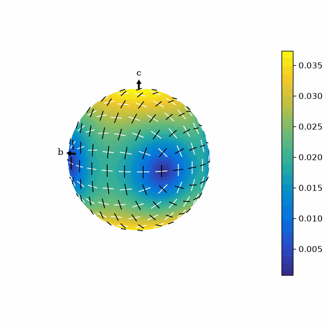
Colour encodes \(\Delta n\) on the unit sphere. The white and black line fields show the fast and slow polarization directions. The response is antipodal: reversing the propagation direction does not change the birefringence.
Optical axes
An optical axis is a propagation direction for which the perpendicular section has equal indices and hence zero birefringence. A biaxial crystal has two such axes. Each axis is a line, so its positive and negative senses are physically equivalent.
vOptical = rI.opticalAxis()
opticalAxisResidual = rI.birefringence(vOptical)[0]
vOptical, opticalAxisResidual
(vector3d (olivine)
  size     : 2
  antipodal: true
       x      y  z
  -0.689  0.725  0
   0.689  0.725  0, array([0., 0.]))
hold(True)
vOptical.antipodal = False
arrow3d(cat(vOptical, -vOptical), faceColor='red')
hold(False)
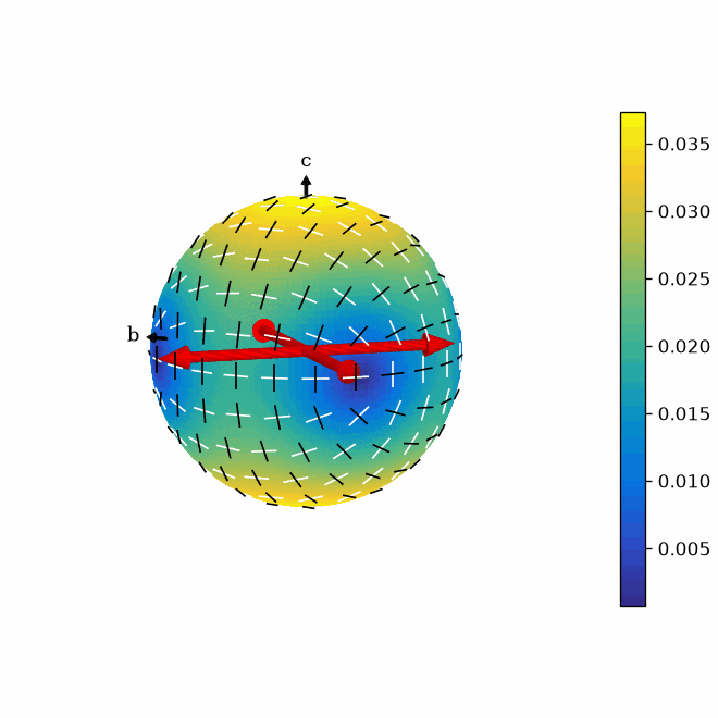
The residual is numerical roundoff rather than physical birefringence. Red arrows mark both senses of both optical axes on the preceding surface. They point at the dark blue minima where \(\Delta n\) falls to zero.
Interference colour between polarizers
An ideal isotropic crystal remains dark between crossed polarizers because it does not change the state of polarization. An anisotropic crystal splits the incident polarization into fast and slow components. Their retardation depends on \(\Delta n\), thickness, and wavelength.
spectralTransmission integrates the transmitted visible spectrum into an RGB triplet. Thickness is specified in nanometres, so 30000 corresponds to 30 micrometres.
vProp = Miller(1, 1, 1, cs)
thickness = 30000
_, pFast, _ = rI.birefringence(vProp)
polarizer = rotation.byAxisAngle(vProp, 30 * degree) * pFast

rgbFromDirection = rI.spectralTransmission(vProp, thickness, polarizationDirection=polarizer)
rgbFromDirection
array([0.2061, 0.5346, 0.6825])
The polarizer above is 30 degrees from the fast direction in the plane perpendicular to
vProp. The same calculation can therefore use tau, the angle between the polarizer
and pMin. The RGB values are fractions on the display colour scale, not measured
intensities.
rgbFromTau = rI.spectralTransmission(vProp, thickness, tau=30 * degree)
rgbFromTau
array([0.2061, 0.5346, 0.6825])
Vary the polarizer angle
With crossed polarizers, the two components have equal magnitude when \(\tau=45\) degrees. The three spherical maps show how the colour and intensity change as the input polarization turns away from the fast axis.
newMtexFigure(layout=[1, 3])

plot(rI.spectralTransmission(thickness, tau=15 * degree), 'rgb')
mtexTitle(r'$\tau = 15^{\circ}$')

nextAxis()
plot(rI.spectralTransmission(thickness, tau=30 * degree), 'rgb')
mtexTitle(r'$\tau = 30^{\circ}$')

nextAxis()
plot(rI.spectralTransmission(thickness, tau=45 * degree), 'rgb')
mtexTitle(r'$\tau = 45^{\circ}$')
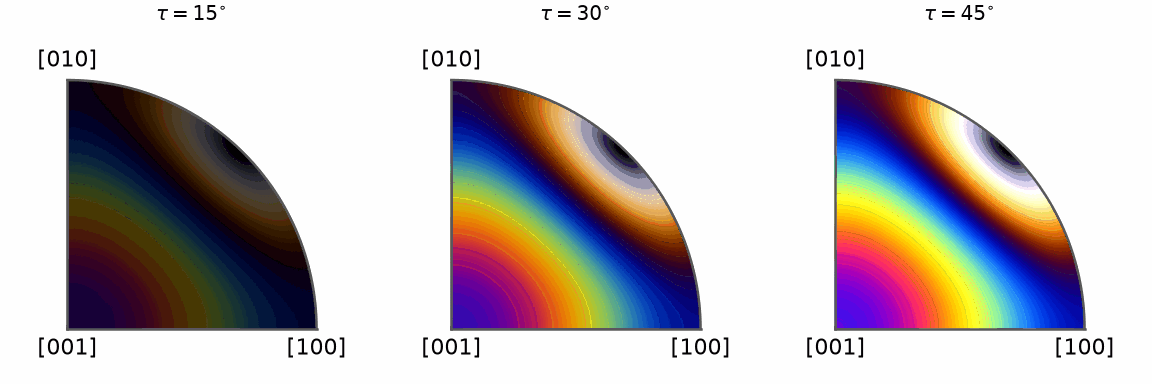
The 45-degree panel is brightest because both permitted waves are excited equally. Directions near an optical axis remain dark in every panel because their retardation is zero.
Vary the analyser angle
The option phi is the angle from the polarizer to the analyser. Crossed polarizers
correspond to \(\phi=90\) degrees. Here tau stays fixed at 45 degrees while the
analyser changes.
newMtexFigure(layout=[1, 3])

plot(rI.spectralTransmission(thickness, tau=45 * degree, phi=30 * degree), 'rgb')
mtexTitle(r'$\phi = 30^{\circ}$')

nextAxis()
plot(rI.spectralTransmission(thickness, tau=45 * degree, phi=60 * degree), 'rgb')
mtexTitle(r'$\phi = 60^{\circ}$')

nextAxis()
plot(rI.spectralTransmission(thickness, tau=45 * degree, phi=90 * degree), 'rgb')
mtexTitle(r'$\phi = 90^{\circ}$')
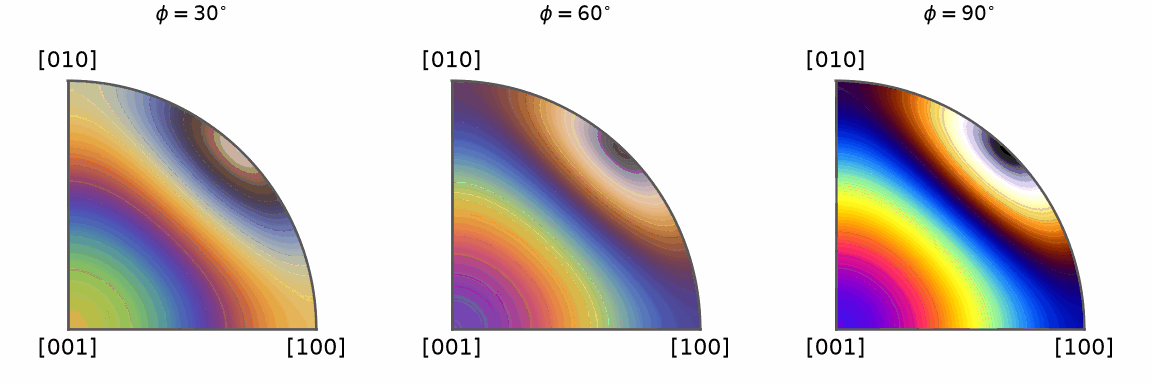
The non-crossed panels retain a bright background that would pass without a crystal. At 90 degrees that background is extinguished, leaving only the wavelength-dependent signal produced by birefringence.
From the crystal frame to the specimen frame
Microscope directions are given in the specimen frame, whereas rI is expressed in the
crystal frame. There are two equivalent calculations. One can rotate the tensor into
every measured crystal orientation, or map the specimen directions back into every
crystal frame.
The simulated section below is 22800 nm thick. Its light propagates along specimen z and its polarizer points along specimen x.
vPropSpecimen = vector3d.Z
polarizerSpecimen = vector3d.X
thickness = 22800
ori = olivine.orientations

# rotate one crystal tensor into every measured orientation
rISpecimen = ori * rI
rgbTensorRoute = rISpecimen.spectralTransmission(vPropSpecimen, thickness, polarizationDirection=polarizerSpecimen)

plot(olivine, rgbTensorRoute)
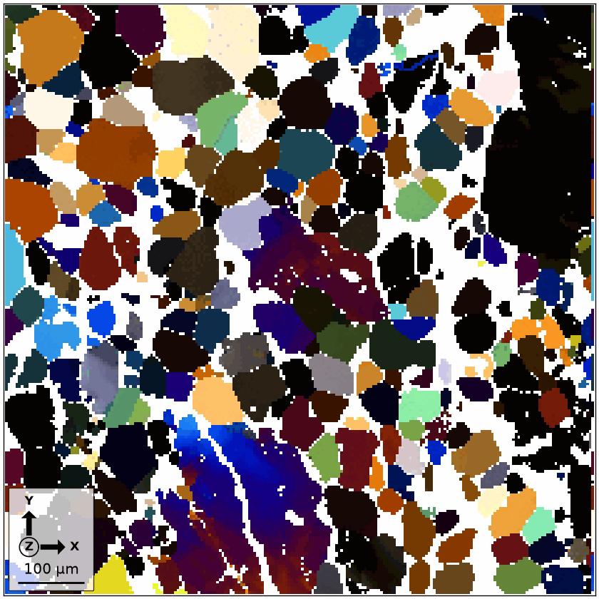
Grains that were merely different IPF colours now acquire colours from the optical model. Within-grain variation follows the measured pixel orientations. The EBSD data supplies orientation only; thickness and composition remain explicit model inputs.
Verify the equivalent direction route
An orientation maps crystal coordinates into specimen coordinates. Its inverse therefore maps each specimen direction into the corresponding crystal frame before applying the original tensor.
vPropCrystal = inv(ori) * vPropSpecimen
polarizerCrystal = inv(ori) * polarizerSpecimen

rgbDirectionRoute = rI.spectralTransmission(vPropCrystal, thickness, polarizationDirection=polarizerCrystal)

# the notIndexed pixels calcGrains gave to olivine grains have no orientation
maxRouteDifference = np.nanmax(np.abs(rgbTensorRoute - rgbDirectionRoute))
maxRouteDifference
3.4217e-13
The notIndexed pixels inside olivine grains, which calcGrains gave the phase of their
grain but no orientation, have no colour and are left out. The maximum channel difference
is at floating-point roundoff. This check is important because plausible colours do not
reveal a reference-frame mistake.
Package the model as a colour key
A spectralTransmissionColorKey stores the tensor, thickness, propagation direction, polarizer, and analyser angle. Its defaults reproduce the specimen-frame setup above.
colorKey = spectralTransmissionColorKey(rI, thickness)
colorKey.propagationDirection = vector3d.Z
colorKey.polarizer = vector3d.X
colorKey.phi = 90 * degree

rgbKey = colorKey.orientation2color(ori)
maxKeyDifference = np.nanmax(np.abs(rgbKey - rgbDirectionRoute))
maxKeyDifference
0
Visualize the colour key
The sigma sections show the colour assigned to orientations throughout orientation space. They are the legend for a map made with this key.
plot(colorKey, 'sigma')
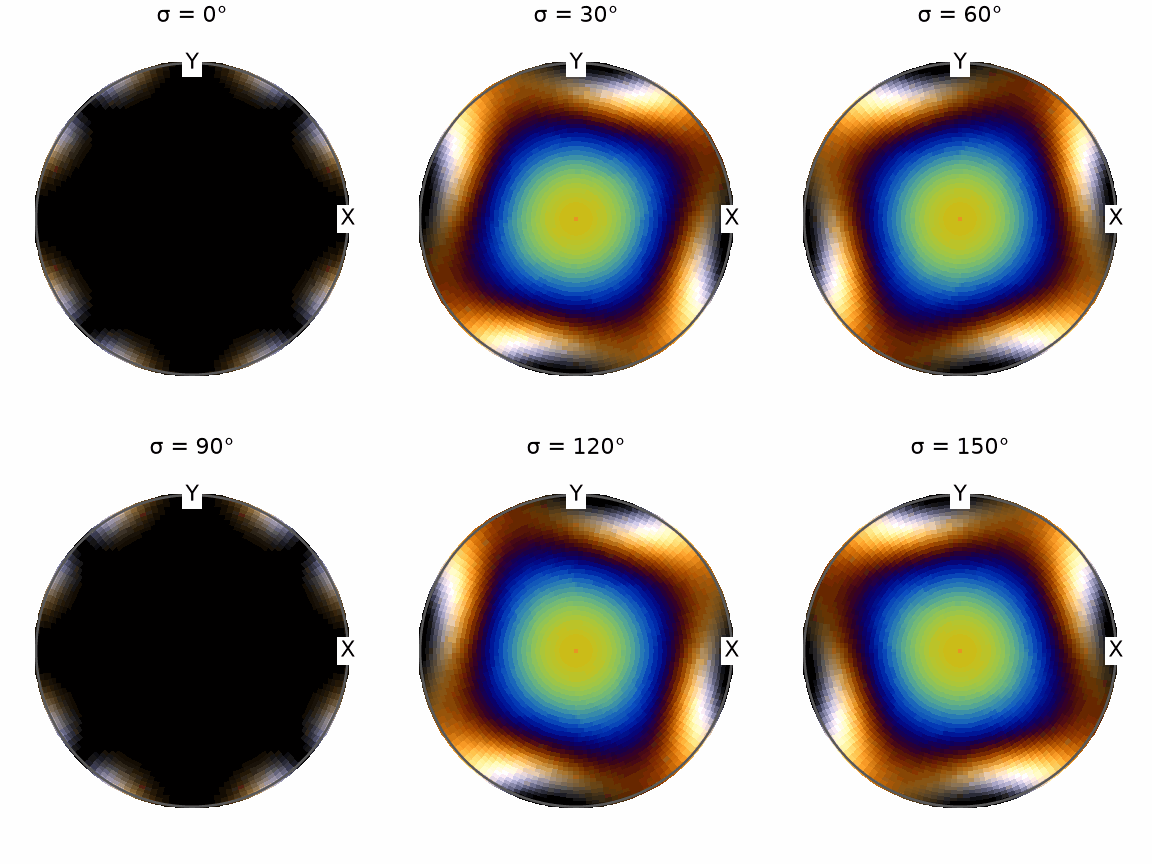
Nearby orientations usually have nearby colours. Rapid changes occur where a small orientation change moves a wavelength through an interference minimum or maximum, so this key is not an IPF key with a different palette.
Circular input polarization
Setting polarizer to None selects the circular-polarization branch of the colour
key. The response then depends on retardation without selecting one linear input
direction in the specimen plane.
colorKey.polarizer = None
rgbCircular = colorKey.orientation2color(ori)

plot(olivine, rgbCircular)
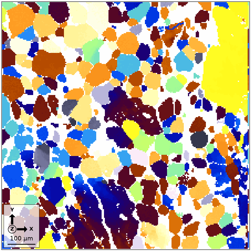
Compared with the linearly polarized map, the circular-input map removes extinction caused only by alignment with a particular polarizer. No grain in this map is fully dark, because none is viewed close enough to an optical axis for its retardation to vanish.
Rotate polarizer and analyser together
Rotating both elements preserves their 90-degree separation while changing their
orientation in the specimen plane. Run in a loop over omega from 0 to 90 degrees, the
map sweeps through a quarter turn. Each grain reaches extinction when a fast or slow
direction aligns with the polarizer. The page draws the frame halfway between
extinction positions.
omega = 45
colorKey.polarizer = rotation.byAxisAngle(vector3d.Z, omega * degree) * vector3d.X
plot(olivine, colorKey.orientation2color(ori), micronbar=False)
mtexTitle(f'{omega:.1f}°')
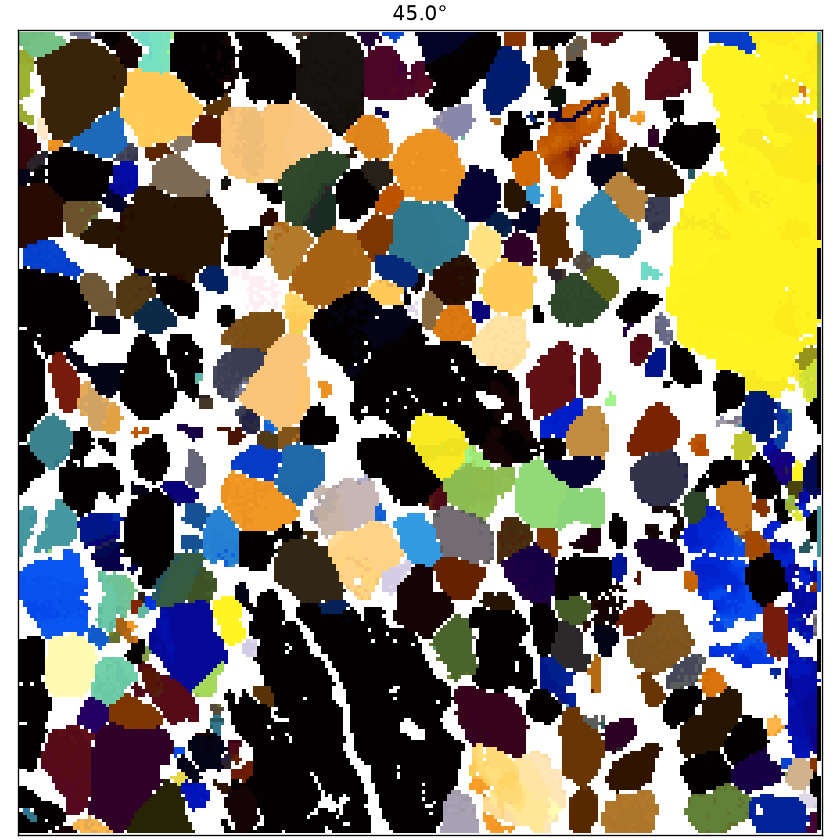
The published frame is left at 45 degrees so the spatial colour variation remains visible. The animation, rather than this final frame alone, shows that different grains reach extinction at different rotation angles.
What the colour model leaves out
This calculation is a qualitative optical simulation. It uses one wavelength-independent refractive-index tensor, a linear Fo-Fa mixture, ideal polarizers, and a CIE colour conversion. It omits dispersion of the principal indices, absorption, scattering, surface effects, illumination, and camera calibration.
Consequently, a matching RGB colour does not by itself validate composition, thickness, or orientation. Those quantities need independent measurements before the result can be compared quantitatively with a microscope image.
The maths behind the interference colour
For a unit propagation direction \(\vec v\), the relevant refractive indices are the two eigenvalues of the tensor section perpendicular to \(\vec v\). Their difference is
\[\Delta n(\vec v)=n_{\mathrm{slow}}(\vec v) -n_{\mathrm{fast}}(\vec v).\]A section of thickness \(t\) produces retardation \(\Gamma=t\Delta n\). At wavelength \(\lambda\), the phase lag is \(2\pi\Gamma/\lambda\). For ideal crossed polarizers the transmitted intensity is proportional to
\[\sin^2(2\tau)\, \sin^2\left(\frac{\pi t\Delta n}{\lambda}\right).\]This explains all three zeros seen above: \(\Delta n=0\) along an optical axis, \(t=0\) for no crystal, and \(\tau=0\) or 90 degrees at extinction.
Next
Magnetic Anisotropy is the next worked physical property in this chapter. Tensor Averages combines rotated single-crystal tensors into aggregate properties. For orientation maps without an optical model, continue with IPF Maps.
Further reading
- J.F. Nye, Physical Properties of Crystals: Their Representation by Tensors and Matrices, Oxford University Press, 1985, develops tensor symmetry and optical properties.
- W.D. Nesse, Introduction to Optical Mineralogy, 4th ed., Oxford University Press, 2013, develops indicatrices, biaxial optics, extinction, and interference colours.
- A. Echalier, R.L. Glazer, V. Fülöp, and M.A. Geday, Assessing crystallization droplets using birefringence, Acta Crystallographica D 60 (2004), 696-702, relates directional birefringence, retardation, optical axes, and crossed polarizers.
- L. Casas, Three-dimensional-printing aids in visualizing the optical properties of crystals, Journal of Applied Crystallography 51 (2018), 901-908, explains uniaxial and biaxial indicatrices and their optical axes.
- Forsterite and Fayalite, Handbook of Mineralogy, Mineral Data Publishing, 2001, give the principal indices and the assignments \(X=b\), \(Y=c\), and \(Z=a\) used above.
- CIE 1931 colour-matching functions, 2 degree observer, International Commission on Illumination, is the standard-observer dataset underlying spectral-to-colour conversion.
Technical Details
The spherical colour maps carry the crystal frame of the tensor, so the port draws them
on the fundamental sector of mmm, a quarter of the disc MATLAB shows; the colours are
the same. The sigma sections of the key are drawn without the arrows MATLAB lays over
them, and the arrows of the optical axes show through the sphere, matplotlib having no
occlusion. The animation of the rotating polarizer is a loop over omega updating the
map; the page draws its last frame.
Citing this page.
This page is part of the documentation of
MTEX, a free and open
source MATLAB toolbox for analyzing and modeling crystallographic textures.
It was written by The MTEX Developers and is published at
https://mtex-toolbox.github.io/BirefringenceDemo_py.html.
If you use MTEX, or reuse text or figures from this page, in your research,
please cite
F. Bachmann, R. Hielscher, H. Schaeben: Texture Analysis with MTEX - Free and Open Source Software Toolbox, Solid State Phenomena 160 (2010), 63-68. 10.4028/www.scientific.net/SSP.160.63
BibTeX
@article{bachmann2010mtex,
  author  = {F. Bachmann and R. Hielscher and H. Schaeben},
  title   = {Texture Analysis with MTEX - Free and Open Source Software Toolbox},
  journal = {Solid State Phenomena},
  volume  = {160},
  pages   = {63-68},
  year    = {2010},
  doi     = {10.4028/www.scientific.net/SSP.160.63},
  url     = {https://doi.org/10.4028/www.scientific.net/SSP.160.63}
}
Other papers describing specific MTEX methods are listed under Publications — please cite the one that best fits your application. The MTEX source code is licensed under the GNU General Public License v2.0; the text and figures of this documentation are licensed under CC BY 4.0, which permits reuse — including by automated systems — provided The MTEX Developers and this page are credited.