Wave Velocities

An elastic disturbance travels through a crystal as three waves. For each propagation direction there is one fast, roughly compressional P-wave and two slower S-waves. Each wave has a speed and a polarisation direction.

Anisotropy makes all six quantities depend on propagation direction. This page computes them from a stiffness tensor, visualises shear-wave splitting, and compares phase velocity with energy velocity.

import matplotlib.pyplot as plt
import numpy as np

from mtex import *

plottingConvention.default('y↑→x')

Load stiffness and density

Use the olivine stiffness tensor introduced in Anisotropic Elasticity. The tensor is in GPa and is expressed in the olivine crystal frame.

fname = mtexdatafile('olivine1997')
cs = crystalFrame('mmm', [4.7646, 10.2296, 5.9942], mineral='Olivine')
C = stiffnessTensor.load(fname, cs)
C

stiffnessTensor (Olivine)
  density: 3.355
  unit   : GPa
  rank   : 4 (3 × 3 × 3 × 3)
  tensor in Voigt matrix representation
  320.5  68.15   71.6   0   0     0
  68.15  196.5   76.8   0   0     0
   71.6   76.8  233.5   0   0     0
      0      0      0  64   0     0
      0      0      0   0  77     0
      0      0      0   0   0  78.7

Wave speed depends on both stiffness and material density \(\rho\). The density of olivine used here is 3.355 g/cm\(^3\). Store it in the tensor because almost every command below needs it.

rho = 3.355
C.density = rho
C

stiffnessTensor (Olivine)
  density: 3.355
  unit   : GPa
  rank   : 4 (3 × 3 × 3 × 3)
  tensor in Voigt matrix representation
  320.5  68.15   71.6   0   0     0
  68.15  196.5   76.8   0   0     0
   71.6   76.8  233.5   0   0     0
      0      0      0  64   0     0
      0      0      0   0  77     0
      0      0      0   0   0  78.7

Density can instead be supplied while constructing the tensor. The corresponding syntax is stiffnessTensor(M, cs, density=rho). It can also be passed as a trailing argument to individual commands. Without density, stiffness alone does not determine a velocity in km/s.

Solve for one propagation direction

The propagation direction \(n\) is normal to the moving wavefront. The polarisation direction gives the particle vibration. velocity returns all three speeds and all three polarisations at once.

n = vector3d.X
vpX, vs1X, vs2X, ppX, ps1X, ps2X = velocity(C, n)
vpX

9.7739

vs1X

4.8433

vs2X

4.7907

ppX

vector3d (Olivine)
  antipodal: true
  x  y  z
  1  0  0

ps1X

vector3d (Olivine)
  antipodal: true
  x  y  z
  0  1  0

ps2X

vector3d (Olivine)
  antipodal: true
  x  y  z
  0  0  1

The outputs are ordered as P-wave, fast S-wave, and slow S-wave. The speeds vpX, vs1X, and vs2X are in km/s. The axes ppX, ps1X, and ps2X give their polarisations. A polarisation is an axis because its sign is arbitrary.

The chosen \(x\) direction is a symmetry axis of the olivine crystal. The three polarisations therefore coincide with coordinate axes. Here the P-wave polarisation is exactly parallel to its propagation.

Solve for a list of directions

The same command accepts any list of propagation directions.

xyz = cat(vector3d.X, vector3d.Y, vector3d.Z)
xyz

vector3d (y↑→x)
  size: 3
  x  y  z
  1  0  0
  0  1  0
  0  0  1

vpXYZ = velocity(C, xyz).vp
vpXYZ

array([9.7739, 7.6531, 8.3425])

Solve over the complete sphere

Omit the propagation direction to compute every direction. The first three outputs are spherical functions. They give P-, fast-S-, and slow-S-wave speed as functions of direction.

The remaining outputs are spherical axis fields. They give the corresponding polarisation at each direction.

vp, vs1, vs2, pp, ps1, ps2 = velocity(C)
vp

S2FunHandle (Olivine)
  bandwidth hint: 32
  antipodal     : true

pp

S2AxisFieldHandle (Olivine)
  bandwidth hint: 32

These are ordinary spherical functions and can be evaluated anywhere.

vpFromGridX = vp.eval(vector3d.X)
vpFromGridX

9.7739

MATLAB’s velocity samples a triangulated grid and interpolates between its nodes, which gives 9.7735 here, a small deviation from the exact vpX above. The functions returned here solve the Christoffel equation at every direction they are evaluated at, so the value is exact.

The option 'harmonic' returns a harmonic expansion instead. Harmonic expansions are smooth and respect crystal symmetry exactly. They are the better choice for three-dimensional plots.

vpHarm = velocity(C, harmonic=True).vp
vpHarm

S2FunHarmonic (Olivine)
  bandwidth: 48
  mean     : 8.439
  antipodal: true

Plot speed and polarisation together

Plot the P-wave speed over the upper hemisphere. Overlay its polarisation axes at sampled propagation directions.

newMtexFigure()
plot(vp, upper=True, complete=True)
hold(True)
plot(pp)
hold(False)
mtexColorMap('blue2red')
mtexColorbar(title='P-wave speed in km/s')

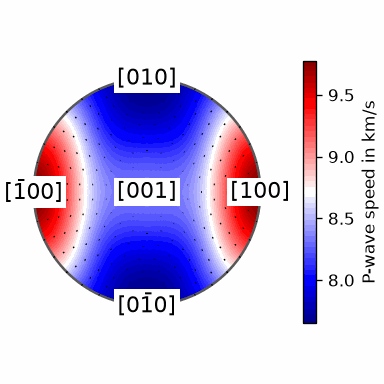
The colour at each point gives speed for that propagation direction. The line segment gives the corresponding particle vibration. Most segments stay close to the radial propagation direction. The P-wave is therefore almost, but not exactly, longitudinal.

See shear-wave splitting

Spherical functions support ordinary arithmetic. Subtract the slow S-wave speed from the fast S-wave speed. Overlay the fast-wave polarisation ps1.

deltaVs = vs1 - vs2

newMtexFigure()
plot(deltaVs, upper=True, complete=True)
hold(True)
plot(ps1)
hold(False)
mtexColorMap('blue2red')
mtexColorbar(title='fast minus slow S-wave speed in km/s')

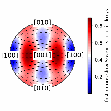
An incident S-wave splits into two perpendicular polarisations. The two components travel at different speeds and arrive with a delay. The line segments show the fast S-wave polarisation measured by a seismologist.

Directions where the speed difference vanishes are acoustic axes. Both S-waves have the same speed there, so no splitting occurs.

Quantify anisotropy

Velocity variation is commonly reported relative to a mean velocity. The convention below uses the midpoint of the fastest and slowest values.

maxVp, maxPos = max(vp)
minVp, minPos = min(vp)
AVp = 200 * (maxVp - minVp) / (maxVp + minVp)
AVp

24.3398

P-wave anisotropy is one number for the complete directional function. Mark the fastest direction with a black square. Mark the slowest direction with a white circle.

S-wave anisotropy compares the two S-waves in each common propagation direction, so it remains a directional function. The ratio of P-wave to fast-S-wave speed is a third useful quantity.

AVs = 200 * (vs1 - vs2) / (vs1 + vs2)

newMtexFigure(layout=[1, 3])

plot(vp, upper=True, axisLabels=False, complete=True)
hold(True)
plot(maxPos, marker='s', markerSize=10, markerFaceColor='k', markerEdgeColor='w')
plot(minPos, marker='o', markerSize=10, markerFaceColor='w', markerEdgeColor='k')
hold(False)
mtexTitle('P-wave speed')

nextAxis()
plot(AVs, upper=True, axisLabels=False, complete=True)
mtexTitle('S-wave anisotropy')

nextAxis()
plot(vp / vs1, complete=True, upper=True, axisLabels=False)
mtexTitle('Vp/Vs1')

mtexColorMap('blue2red')

# one call with one title per panel - repeated calls toggle the colorbars off
mtexColorbar(title=['km/s', 'percent', 'ratio'])

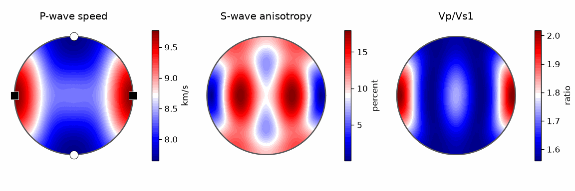
The first map locates the directions behind the scalar AVp. The second map is zero on acoustic axes and largest where splitting is strongest. The third map is dimensionless and need not have extrema in the same directions as either speed alone.

Compare with an isotropic aggregate

Average randomly oriented olivine crystals with a uniform ODF. mean gives the Voigt average. Isotropic Theory defines the Voigt, Reuss, and Hill alternatives and explains why the exact aggregate stiffness is bounded.

C_iso = mean(C, uniformODF(cs))
C_iso

stiffnessTensor (y↑→x)
  density: 3.355
  unit   : GPa
  rank   : 4 (3 × 3 × 3 × 3)
  tensor in Voigt matrix representation
   237.56  78.4867  78.4867        0        0        0
  78.4867   237.56  78.4867        0        0        0
  78.4867  78.4867   237.56        0        0        0
        0        0        0  79.5367        0        0
        0        0        0        0  79.5367        0
        0        0        0        0        0  79.5367

This average is elastically isotropic. Its wave speeds are independent of propagation direction. They are determined completely by bulk modulus \(K\), shear modulus \(G\), and density.

K = C_iso.bulkModulus()
G = C_iso.shearModulus()

vpIso = np.sqrt((K + 4 / 3 * G) / rho)
vpIso

8.4147

vsIso = np.sqrt(G / rho)
vsIso

4.8690

These formulas agree with velocity for the isotropic tensor.

vp_iso, vs1_iso, vs2_iso, *_ = velocity(C_iso, vector3d.X)
vp_iso

8.4147

vs1_iso

4.8690

vs2_iso

4.8690

Both isotropic S-waves have the same speed. An isotropic medium therefore has no shear-wave splitting. Place its P-wave speed between the single-crystal extremes.

cprintf([minVp, vpIso, maxVp], '-Lc', ['min Vp', 'isotropic', 'max Vp'])

   min Vp isotropic    max Vp
  7.65306   8.41473    9.7739

Compare phase velocity with energy velocity

The computed speeds are phase velocities. Phase velocity describes how fast a wavefront moves along its normal \(n\).

Energy travels along the energy velocity vector \(V_e\). In a lossless medium this is a good proxy for group velocity. energyVector computes it from the stiffness, propagation direction, phase speed, and polarisation.

# an arbitrary, non-symmetry propagation direction
nOblique = vector3d.byPolar(45 * degree, 20 * degree)

vpOblique, vs1Oblique, vs2Oblique, ppOblique, ps1Oblique, ps2Oblique = velocity(C, nOblique)

Ve = energyVector(C, nOblique, vpOblique, ppOblique)
Ve

vector3d (Olivine)
     x     y     z
  6.92  1.57  5.11

In an anisotropic medium, \(V_e\) is generally not parallel to \(n\). The energy is deflected sideways by the following angle in degrees.

energyDeflection = angle(Ve, nOblique) / degree
energyDeflection

10.7498

The magnitude of \(V_e\) is at least as large as the phase velocity. Its projection onto \(n\) reproduces the phase velocity exactly.

cprintf([norm(Ve), dot(Ve, nOblique), vpOblique], '-Lc', ['|Ve|', 'Ve.n', 'Vp'])

   |Ve|    Ve.n      Vp
8.74413 8.59068 8.59068

Passing an empty propagation direction with spherical speed and polarisation functions returns a spherical vector field.

VeField = energyVector(C, None, vp, pp)
VeField

S2VectorFieldHandle (Olivine)
  bandwidth hint: 32

Plot phase-velocity and slowness surfaces

A phase-velocity surface places each speed at a radial distance from the origin. A slowness surface uses reciprocal speed in s/km. Plot sections through the plane with normal \(x\).

planeNormal = vector3d.X

# common section and arrow options
optSec = dict(color='interp', lineWidth=6)
optQuiver = dict(lineWidth=2, autoScaleFactor=0.35)
optQuiverProp = dict(color='k', lineWidth=2, autoScaleFactor=0.25)
prop = S2VectorFieldHarmonic.normal()

newMtexFigure(layout=[1, 2])

# phase velocities
plotSection(vp, planeNormal, **optSec, displayName='Vp')
hold(True)
plotSection(vs1, planeNormal, **optSec, displayName='Vs1')
plotSection(vs2, planeNormal, **optSec, displayName='Vs2')

# polarisation directions
quiverSection(vp, pp, planeNormal, color='c', **optQuiver, displayName='pp')
quiverSection(vs1, ps1, planeNormal, color='g', **optQuiver, displayName='ps1')
quiverSection(vs2, ps2, planeNormal, color='m', **optQuiver, displayName='ps2')

# propagation directions as reference
quiverSection(vp, prop, planeNormal, **optQuiverProp, displayName='n')
quiverSection(vs1, prop, planeNormal, **optQuiverProp)
quiverSection(vs2, prop, planeNormal, **optQuiverProp)
hold(False)
mtexTitle('Phase velocity surface')

nextAxis()

# slowness surfaces
plotSection(1 / vp, planeNormal, **optSec, displayName='Vp')
hold(True)
plotSection(1 / vs1, planeNormal, **optSec, displayName='Vs1')
plotSection(1 / vs2, planeNormal, **optSec, displayName='Vs2')

# polarisation directions
quiverSection(1 / vp, pp, planeNormal, color='c', **optQuiver, displayName='pp')
quiverSection(1 / vs1, ps1, planeNormal, color='g', **optQuiver, displayName='ps1')
quiverSection(1 / vs2, ps2, planeNormal, color='m', **optQuiver, displayName='ps2')

# propagation directions as reference
quiverSection(1 / vp, prop, planeNormal, **optQuiverProp, displayName='n')
quiverSection(1 / vs1, prop, planeNormal, **optQuiverProp)
quiverSection(1 / vs2, prop, planeNormal, **optQuiverProp)
hold(False)
legend('Vp', 'Vs1', 'Vs2', 'pp', 'ps1', 'ps2', 'n', location='eastOutside')
mtexTitle('Slowness surface')

mtexColorMap('blue2red')
mtexColorbar(title=['km/s', 's/km'], location='southOutside')

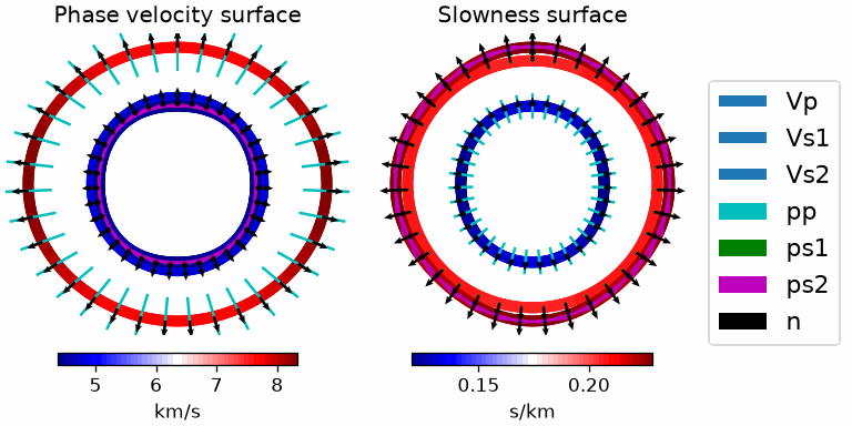
In both panels, the black arrows show propagation direction. The coloured arrows show the three polarisations.

The view looks along the section normal \(x\). Every propagation direction in this plane has its fast S-wave polarised exactly along \(x\), so the green ps1 arrows point straight at the reader and project to a point. The legend still lists ps1, but only the cyan pp and the magenta ps2 arrows have a length on screen, and both lie in the section plane.

The phase panel is longest where a wave is fastest. The slowness panel is longest where that same wave is slowest.

Use the overview plot

plotSeismicVelocities collects the main velocity, anisotropy, ratio, and polarisation maps.

plotSeismicVelocities(C)

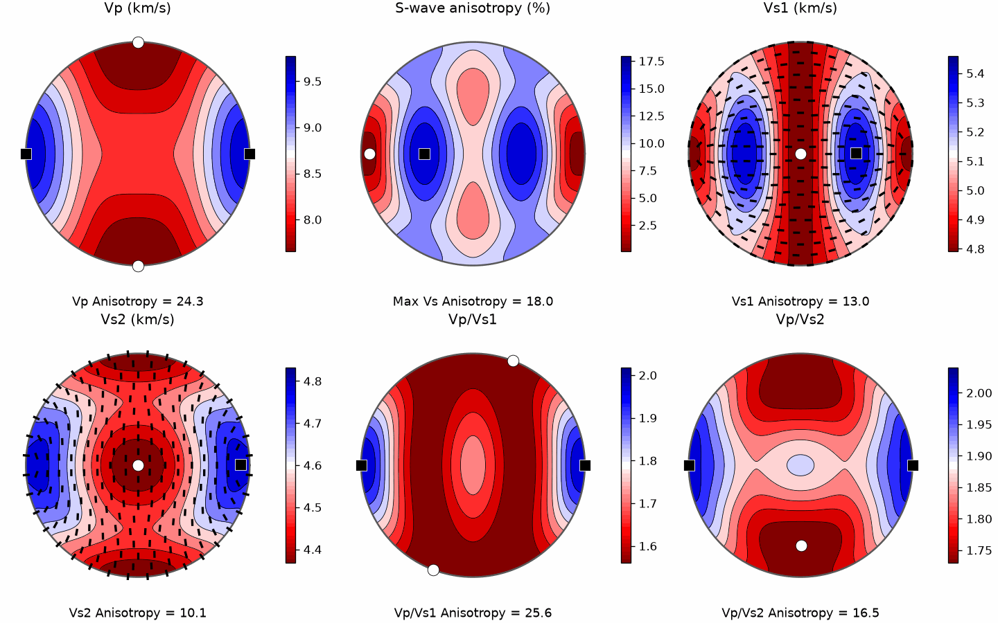
Read the panels together: extrema in one wave need not coincide with extrema in splitting or in a velocity ratio.

The maths behind the wave speeds

Consider a plane wave with propagation direction \(n\), phase velocity \(v\), and polarisation \(p\). Its displacement field has the form

Insert this trial wave into the equation of motion \(\rho\,\partial_t^2u_i=\partial_j\sigma_{ij}\). Use Hooke’s law \(\sigma_{ij}=C_{ijkl}\varepsilon_{kl}\) from Anisotropic Elasticity. The result is the Christoffel equation

The rank-two tensor \(T_{ik}(n)=C_{ijkl}n_jn_l\) is the Christoffel tensor. ChristoffelTensor computes it for a chosen propagation direction.

T = ChristoffelTensor(C, vector3d.X)
T

ChristoffelTensor (Olivine)
  density: 3.355
  rank   : 2 (3 × 3)
  320.5     0   0
      0  78.7   0
      0     0  77

The symmetry \(C_{ijkl}=C_{klij}\) makes \(T\) symmetric. Its three eigenvalues are therefore real and its eigenvectors are mutually perpendicular. Positive-definite stiffness also makes all three eigenvalues positive. They correspond to three real wave speeds.

lam, pEigen = eig(T)
pEigen

vector3d (Olivine)
  size     : 3
  antipodal: true
  x  y  z
  0  0  1
  0  1  0
  1  0  0

lam

array([ 77. ,  78.7, 320.5])

MTEX returns these eigenvalues in ascending order. Divide by density and take square roots to recover speeds in km/s.

vEigen = np.sqrt(lam / rho)
vEigen

array([4.7907, 4.8433, 9.7739])

The largest value belongs to the P-wave, whose polarisation is closest to the propagation direction. The two smaller values belong to the fast and slow S-waves. The earlier call to velocity performs this decomposition and sorting automatically.

References

• E. H. Abramson, J. M. Brown, L. J. Slutsky, and J. Zaug, The elastic constants of San Carlos olivine to 17 GPa, Journal of Geophysical Research 102(B6) (1997), 12253-12263, provides the olivine stiffness tensor used here.
• F. I. Fedorov, Theory of Elastic Waves in Crystals, Plenum Press, New York, 1968, derives the energy-velocity expression implemented by energyVector.

Next

Seismic Properties of Polycrystals applies this workflow to measured preferred orientations. It averages the crystal tensors and interprets the aggregate seismic anisotropy.

Technical Details

MATLAB’s addOption(C, 'density', rho) is the assignment C.density = rho; the loader already reads the density 3.355 g/cm\(^3\) the olivine file states. velocity returns its six outputs as one named tuple, so a single output is picked by name, velocity(C, xyz).vp, where MATLAB takes the first. Without a direction the speeds and polarisations are functions solving the Christoffel equation wherever they are evaluated, where MATLAB interpolates on a triangulated grid of 18338 nodes; so the extremes are exact, 7.65306 and 9.7739 km/s for MATLAB’s 7.65328 and 9.7735, and the P-wave anisotropy is 24.3398 for MATLAB’s 24.3329. The extremes of an antipodal function are axes, so the markers of the maximum and the minimum appear at both of their ends on the rim, where MATLAB marks one. eig returns the eigenvalues first. S2VectorFieldHarmonic.normal() is MATLAB’s static method with its parentheses.

@article{bachmann2010mtex,
  author  = {F. Bachmann and R. Hielscher and H. Schaeben},
  title   = {Texture Analysis with MTEX - Free and Open Source Software Toolbox},
  journal = {Solid State Phenomena},
  volume  = {160},
  pages   = {63-68},
  year    = {2010},
  doi     = {10.4028/www.scientific.net/SSP.160.63},
  url     = {https://doi.org/10.4028/www.scientific.net/SSP.160.63}
}