Symmetric spherical functions

A symmetric spherical function has the same scalar value at directions related by a point group. Inverse pole figures and directional properties of a single crystal are common examples. MTEX represents a harmonic function with this constraint as an S2FunHarmonic whose reference frame carries the point group.

Symmetry is the point group under which the data is invariant. It is attached to a reference frame rather than being a reference frame itself. Use a specimenFrame for directions in the specimen frame and a crystalFrame for directions in a crystal frame.

import numpy as np

from mtex import *

plottingConvention.default('y↑→x')

Attach and enforce a symmetry

Start with an ordinary harmonic spherical function. The asymmetric smiley makes the effect of symmetrisation easy to see.

sF = S2Fun.smiley()

Choose orthorhombic specimen symmetry. Passing sF.how2plot preserves the plotting convention of the function when the symmetry creates its reference frame.

ss = specimenFrame('222', sF.how2plot)

symmetrise attaches the symmetry and its frame, averages symmetry-related directions and so enforces the constraint.

sFs1 = symmetrise(sF, ss)

Plot the fundamental sector

A symmetric function is plotted only in a representative sector by default, as is usual for an inverse pole figure.

plot(sFs1)

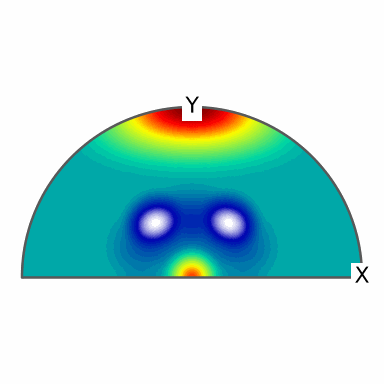
This sector contains one representative from each set of directions related by 222 symmetry. Its boundaries therefore remove repeated information; they do not crop the definition of the function.

Inspect the full symmetrised function

Use complete when the repetitions themselves matter. The upper option restricts the view to the upper hemisphere.

plot(sFs1, complete=True, upper=True)

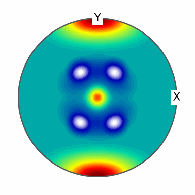
The smiley motif now occurs in positions related by the half-turns of 222 symmetry. All copies have identical values, although their positions and orientations on the projection differ.

Construct from a function

A Python function is convenient when values can be computed for every direction. It must accept a vector3d array and return one real scalar per direction. Here the directions belong to the crystal frame, so the requested point group is crystal symmetry 6/m.

valueFunction = lambda v: 0.1 * (v.theta + np.sin(8 * v.x) * np.sin(8 * v.y))
cs = crystalFrame('6/m')

quadrature computes the harmonic coefficients and enforces the supplied symmetry. The bandwidth option keeps spherical harmonic degrees through 16.

sFs2 = S2FunHarmonic.quadrature(valueFunction, cs, bandwidth=16)

contour(sFs2, lineWidth=2)
mtexColorMap('parula')

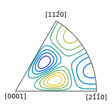
Only the fundamental sector of 6/m is drawn. The curved contour lines are the part of the scalar function that is not generated by symmetry; applying the point group reproduces them over the complete sphere.

The maths behind symmetrisation

For a point group \(G\), symmetrisation replaces a function \(f\) by the group average

Applying any group element merely permutes the terms in this sum. The result therefore satisfies \(f_G(g\vec v)=f_G(\vec v)\) for every \(g\) in \(G\). The harmonic implementation performs this averaging while keeping a compact coefficient representation.

References

• H.-J. Bunge, Texture Analysis in Materials Science: Mathematical Methods, Butterworths, 1982, develops the crystal and specimen symmetry operations that reduce directional texture information to a representative region.

Next

Continue with Convolution to see how a function on the rotation group acts on a spherical function.

Technical Details

The port has no S2FunHarmonicSym: a frame carries its point group, so an S2FunHarmonic in a frame with symmetry is the symmetric function. MATLAB’s two steps, S2FunHarmonicSym(sF, ss) attaching the frame and symmetrise averaging, are the one call symmetrise(sF, ss), since a function whose frame claims a symmetry it does not have is not a state the port admits. MATLAB’s clf before a plot has no counterpart; every plot opens its own figure.

The sector of 222 holds a quarter of the sphere, the half \(y \ge 0\) of a hemisphere. In MATLAB symmetrise returns a plain S2FunHarmonic again, and its plot shows the octant \(x, y, z \ge 0\), half of that sector; the symmetrised smiley is not antipodal, so the octant does not show every value.

@article{bachmann2010mtex,
  author  = {F. Bachmann and R. Hielscher and H. Schaeben},
  title   = {Texture Analysis with MTEX - Free and Open Source Software Toolbox},
  journal = {Solid State Phenomena},
  volume  = {160},
  pages   = {63-68},
  year    = {2010},
  doi     = {10.4028/www.scientific.net/SSP.160.63},
  url     = {https://doi.org/10.4028/www.scientific.net/SSP.160.63}
}