Spherical Approximation and Interpolation

A set of measured directions and values does not yet define a function between the measurements. Interpolation fills those gaps while preserving every measured value. Approximation permits small residuals at the measured directions in exchange for a simpler or smoother function.

import numpy as np

from mtex import *

plottingConvention.default('y↑→x')

Load scattered values

The example data contain directions on the sphere and one scalar value at each direction. The first three columns are Cartesian components of the directions. The fourth column contains the values. We import them with loadVector3d, whose second output S is a dict with an entry S['values'] holding that fourth column.

fname = mtexdatafile('smiley')
nodes, S = loadVector3d(fname, columnNames=['x', 'y', 'z', 'values'])
values = S['values']

A scatter plot shows only the measured directions. It does not make any claim about the values between them.

scatter(nodes, values, upper=True)

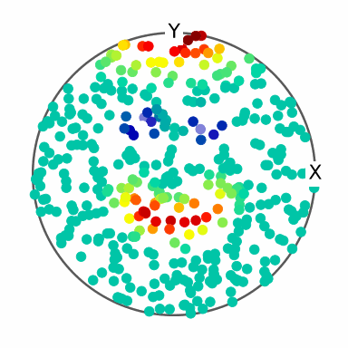
Notice the eyes and curved mouth encoded by the coloured samples. Large spaces between samples are precisely where a reconstruction method must supply information that was not measured.

Exact interpolation

An interpolant agrees exactly with every supplied value. With the 'linear' method, MTEX triangulates the directions and varies the value linearly over each spherical triangle. This is the spherical counterpart of joining samples in a one-dimensional plot by straight segments.

sFTri = interp(nodes, values, 'linear')

The result is an S2FunTri. Evaluate it at the original directions to test the defining interpolation property.

linearError = np.linalg.norm(sFTri.eval(nodes) - values)
linearError

1.1088e-15

The residual norm is at machine precision. The function therefore matches the data at the nodes, but this test says nothing about the gaps.

newMtexFigure()
contourf(sFTri, upper=True)

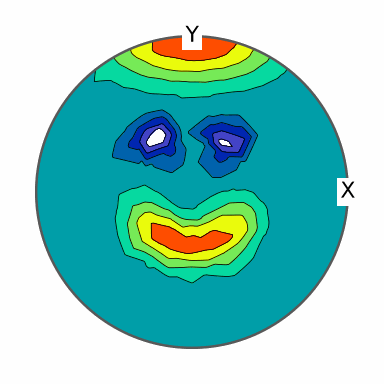
The triangulated surface does not recover the intended happy face cleanly. Exact agreement at the nodes has not guaranteed a plausible shape between them. Other gap-filling variants can preserve the interpolation property and may improve the result, but they must make a different local choice.

Smooth harmonic approximation

An approximation is not constrained to reproduce every supplied value. Here a truncated series of spherical harmonics (Basics of spherical harmonics) describes the whole sphere with fewer coefficients than there are samples. The resulting least-squares problem is overdetermined, so the fit generally has nonzero residuals.

sF = interp(nodes, values, 'harmonic')

The 'harmonic' option returns an S2FunHarmonic. Its default bandwidth is chosen from the number of nodes.

newMtexFigure()
contourf(sF, upper=True)

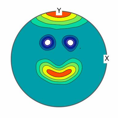
The harmonic plot is much smoother, and the eyes and smile form coherent features rather than following individual triangles. Smoothing has traded exact agreement at the data nodes for a simpler global description.

harmonicError = np.linalg.norm(sF.eval(nodes) - values)
harmonicError

0.0605

This residual is not zero, unlike the interpolation residual. Such a trade can be useful when the measured values contain noise and the unknown exact function values should not be reproduced point for point.

Choosing between the two results

Use interpolation when each supplied value is authoritative and values at unsampled directions should be inferred locally. Use harmonic approximation when the data are noisy or when a smooth global representation is the goal. In either case, inspect both the residuals at the nodes and the behaviour between them. A small residual alone does not validate the reconstructed shape.

The maths behind harmonic approximation

Let \(x_n\), \(n=1,\ldots,N\), denote the data directions and let \(f(x_n)\) be their values. A harmonic approximation of maximum degree \(M\) has the form

The values \(\hat f_m^l\) are the Fourier coefficients. With fewer harmonic coefficients than data values, they can be found from the least-squares problem

This equation states the basic unweighted strategy. By default, S2FunHarmonic.interpolate applies spherical Voronoi weights so that densely sampled areas do not dominate the fit merely because they contain more nodes.

The LSQR solver obtains the coefficients iteratively. The optimality condition is the normal equation, but MTEX need not store the Fourier matrix explicitly. That matrix would be

Each solver iteration needs products with this matrix or its adjoint. MTEX evaluates these products efficiently with the nonequispaced spherical Fourier transform (NFSFT). The final Fourier coefficients completely describe the approximation \(g\).

References

• J. Keiner, S. Kunis and D. Potts, NFSFT software and documentation, describes the nonequispaced spherical Fourier transform used for the harmonic matrix-vector products.

Next

Continue with Sampling to learn how a continuous spherical function is replaced by weighted values at selected directions.

Technical Details

vector3d.load returns the directions alone; loadVector3d returns them with the dict of the other columns, MATLAB’s second output. The sample file is fetched on first use by mtexdatafile('smiley'), where MATLAB reads it from mtexDataPath. The products with the Fourier matrix are finufft’s nonuniform FFTs here, MATLAB’s lsqr the port’s own LSQR; the residual is 0.0605 where MATLAB’s is 0.0606.

@article{bachmann2010mtex,
  author  = {F. Bachmann and R. Hielscher and H. Schaeben},
  title   = {Texture Analysis with MTEX - Free and Open Source Software Toolbox},
  journal = {Solid State Phenomena},
  volume  = {160},
  pages   = {63-68},
  year    = {2010},
  doi     = {10.4028/www.scientific.net/SSP.160.63},
  url     = {https://doi.org/10.4028/www.scientific.net/SSP.160.63}
}