Sampling a Spherical Function

A spherical density is a nonnegative S2Fun whose values describe how mass is distributed over directions. Some computations need that density replaced by finitely many directions. Examples include simulation input, numerical integration, and a scatter plot of likely directions.

MTEX can draw directions independently or optimize their placement. It can also attach a volume fraction to every optimized direction. This page compares those three choices and tests what each sample preserves.

import matplotlib.pyplot as plt
import numpy as np

from mtex import *

plottingConvention.default('y↑→x')

A density with narrow features

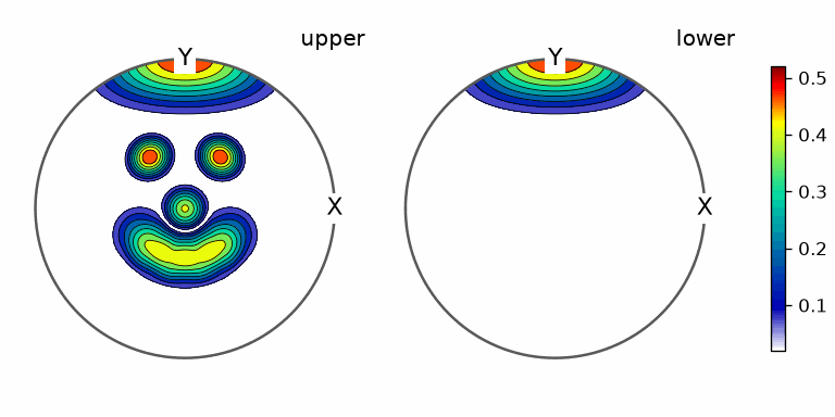
The example is the smiley function. Its underlying features are zero on most of the sphere and concentrated in the eyes and mouth. The constant background below makes the density strictly positive without hiding those narrow features.

sF = 0.02 + abs(S2Fun.smiley())

contourf(sF)
mtexColorbar()

Random sampling

discreteSample draws independent directions with probability proportional to the function value. It is fast and unbiased, but a finite random sample contains clusters and empty patches.

vRnd = discreteSample(sF, 1000)

contourf(sF)
hold(True)
scatter(vRnd, markerSize=4, markerFaceColor='k', markerEdgeColor='k')
hold(False)

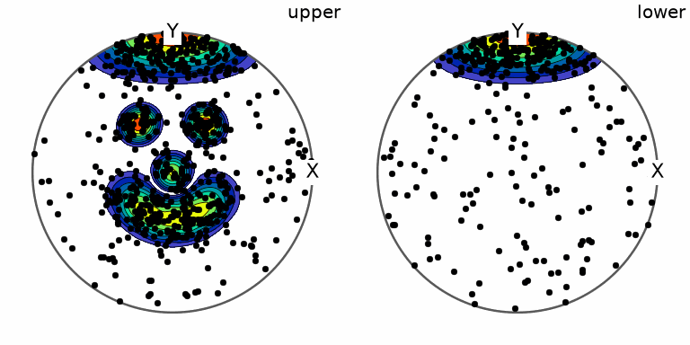
Notice the uneven gaps between points along the mouth. Those gaps are sampling noise rather than low-density parts of the original function.

Optimizing the directions

optimalSample moves the directions until their discrete measure is close to the density. This optimization costs more time than independent sampling. In return, the directions spread evenly along every feature and become denser where the function is large.

vOpt = optimalSample(sF, 1000, bandwidth=128)

contourf(sF)
hold(True)
scatter(vOpt, markerSize=4, markerFaceColor='k', markerEdgeColor='k')
hold(False)

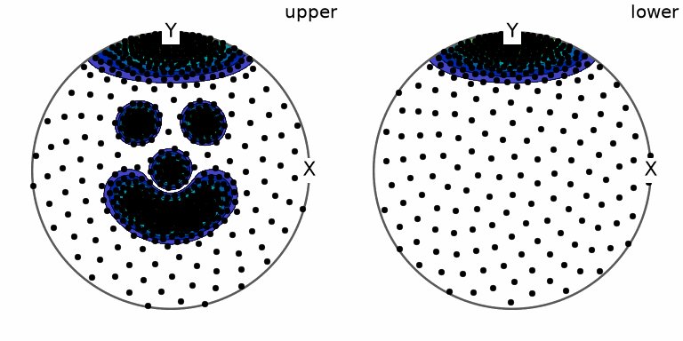
The optimized sample follows both eyes and the mouth without the random clusters seen above. Because this example has a positive background, a few directions also remain away from those features.

The bandwidth sets the largest harmonic degree that the sample must reproduce. Choose it for the intended use of the points. A lower bandwidth asks the optimizer to preserve less detail and is faster.

Optimizing directions and weights

The points do not have to carry equal mass. Asking optimalSample for the weights, optimizeWeights=True, optimizes them together with the directions. For \(M\) directions, this gives the discrete measure \(M\) additional variables.

vWgt, c = optimalSample(sF, 100, bandwidth=32, optimizeWeights=True)

The weights are volume fractions. They are nonnegative and sum to one. The output below checks both properties for this sample.

np.array([np.min(c), np.max(c), np.sum(c)])

array([0.0056, 0.0189, 1.    ])

Marker area now follows the weight. A large marker represents a direction that carries a larger share of the density.

contourf(sF)
hold(True)
scatter(vWgt, markerSize=40 * c / np.mean(c), markerFaceColor='k', markerEdgeColor='k')
hold(False)

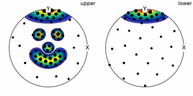
Notice that the directions remain well distributed, but their shares are no longer equal. Directions with almost no mass can be discarded during the optimization by passing the minWeight option.

We use 100 points and bandwidth 32 so that the weights have visible work to do. With 500 points and bandwidth 128, the optimized directions already describe this density so well that the weights in a measured run ranged only from 0.0019605 to 0.0019609.

Comparing the recovered densities

To compare equal point counts, we estimate a density from every sample with calcDensity. The weighted sample passes its volume fractions to the estimator. All three estimates use the same kernel halfwidth, so their smoothing is identical.

A second error compares the spherical harmonic coefficients of the discrete measure directly through degree 32. No smoothing kernel enters this test. This is the coefficient discrepancy that optimalSample actually minimizes, although its restricted-distance objective assigns a degree-dependent weight to each coefficient. The unweighted relative norm below is easier to interpret when the sample will be used for integration.

hw = 5 * degree
sFn = sF / mean(sF)
sF32 = S2FunHarmonic(sF, bandwidth=32)

dens = lambda v, w: norm(calcDensity(v, weights=w, halfwidth=hw) - sFn)
mom = lambda v, w: norm(sum(sF) * S2FunHarmonic.adjointNFSFT(v, w / np.sum(w), bandwidth=32) - sF32) / norm(sF32)

M = [50, 100, 200, 400, 800]
densRnd, densOpt, densWgt = np.zeros(len(M)), np.zeros(len(M)), np.zeros(len(M))
momRnd, momOpt, momWgt = np.zeros(len(M)), np.zeros(len(M)), np.zeros(len(M))

for k, m in enumerate(M):

  # average the random result over three independent draws
  d, e = np.zeros(3), np.zeros(3)
  for r in range(3):
    v = discreteSample(sF, m)
    d[r] = dens(v, np.ones(m))
    e[r] = mom(v, np.ones(m))
  densRnd[k], momRnd[k] = np.mean(d), np.mean(e)

  v = optimalSample(sF, m, bandwidth=32)
  densOpt[k] = dens(v, np.ones(v.size))
  momOpt[k] = mom(v, np.ones(v.size))

  v, w = optimalSample(sF, m, bandwidth=32, optimizeWeights=True)
  densWgt[k] = dens(v, w)
  momWgt[k] = mom(v, w)

names = ['points', 'densityRandom', 'densityOptimal', 'densityWeighted', 'momentRandom', 'momentOptimal', 'momentWeighted']
print(''.join(f'{n:>17s}' for n in names))
for row in zip(M, densRnd, densOpt, densWgt, momRnd, momOpt, momWgt):
  print(f'{row[0]:>17d}' + ''.join(f'{x:>17.4f}' for x in row[1:]))

           points    densityRandom   densityOptimal  densityWeighted     momentRandom    momentOptimal   momentWeighted
               50           1.8483           1.0790           1.0738           2.4475           2.0445           2.0861
              100           1.4049           0.6570           0.5339           1.7759           0.9897           0.9171
              200           1.0007           0.4387           0.3058           1.2691           0.5699           0.3510
              400           0.7053           0.3017           0.2536           0.9066           0.3307           0.2280
              800           0.5510           0.2450           0.2343           0.6215           0.1784           0.0909

plt.figure()
plt.loglog(M, densRnd, '-o', M, densOpt, '-s', M, densWgt, '-d', linewidth=2, markersize=8)
legend('discreteSample', 'optimalSample', 'optimalSample, weighted')
plt.xlabel('number of sampling points')
plt.ylabel('L^2 error of the recovered density')

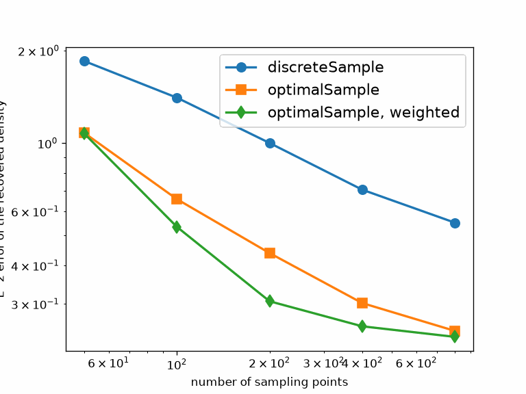
At every equal point count, an optimized sample recovers the density more accurately than the random sample. Two hundred optimized points have an error of 0.44, less than the about 0.5 of 800 random points. At 100 points the weighted optimization reduces the error from about 0.66 to about 0.53.

The optimized curves flatten near 0.24, while the random curve is still descending. Their flattening shows that the 5 degree kernel is becoming a limiting source of error for this sharp function.

plt.figure()
plt.loglog(M, momRnd, '-o', M, momOpt, '-s', M, momWgt, '-d', linewidth=2, markersize=8)
legend('discreteSample', 'optimalSample', 'optimalSample, weighted')
plt.xlabel('number of sampling points')
plt.ylabel('error of the harmonic coefficients up to degree 32')

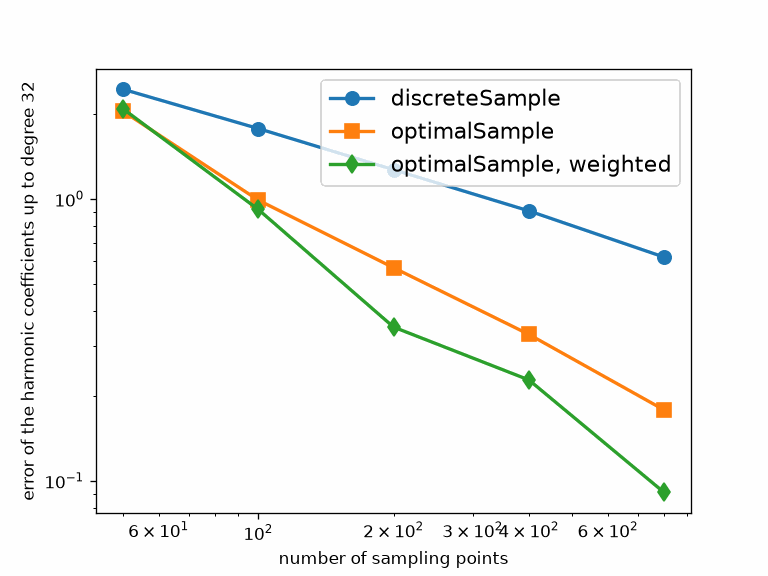
Without the smoothing kernel there is no common floor. The optimized samples converge more quickly, while random sampling has the familiar \(1/\sqrt{M}\) statistical rate. At 50 points, changing the weights gives essentially no benefit because the directions use most of what this small sample can express.

At 800 points, the weighted sample has a coefficient error of 0.09. This is about seven times more accurate than the random sample and twice as accurate as the unweighted optimized sample.

Choosing a sampling method

Use discreteSample when you need many points quickly and their individual placement does not matter. Use optimalSample when the number of points is limited. Ask for weights when the sample will be used for integration. For a kernel density estimate, optimized weights usually help less once the smoothing halfwidth becomes the main source of error.

The maths behind the optimized sample

Directions \(\mathbf{v}_j\) and volume fractions \(c_j\) represent the density \(f\) by the discrete measure

Here \(\delta_{\mathbf{v}_j}\) places mass at one direction. The weights satisfy \(c_j\geq 0\) and \(\sum_j c_j=1\). The optimizer moves the directions and, when requested, the weights to reduce harmonic discrepancies through the chosen bandwidth.

References

• M. Gräf, D. Potts and G. Steidl, Quadrature Errors, Discrepancies, and Their Relations to Halftoning on the Torus and the Sphere, SIAM Journal on Scientific Computing 34 (2012), A2760–A2791, develops the discrepancy measure used to optimize discrete samples on the sphere.
• M. Knezevic and N. W. Landry, Procedures for reducing large datasets of crystal orientations using generalized spherical harmonics, Mechanics of Materials 88 (2015), 73–86, applies harmonic moment matching to compact directional datasets.

Next

Continue with Harmonic Representation to see how bandwidth and spherical harmonic coefficients describe the detail that these optimized samples are designed to preserve.

Technical Details

MATLAB’s second output [v, c] = optimalSample(...) is optimizeWeights=True here. norm is that of the normalised measure, \(1/\sqrt{4\pi}\) times MATLAB’s, so the density errors are \(1/\sqrt{4\pi}\) of MATLAB’s (0.44 for MATLAB’s 1.51, 0.66 and 0.53 for its 2.28 and 1.82); the coefficient errors are ratios and compare directly, 0.092, 0.181 and 0.622 at 800 points for MATLAB’s 0.101, 0.185 and 0.617. The random columns differ from run to run. MATLAB’s page also compares its table with the numbers of an earlier run, which this page leaves out.

@article{bachmann2010mtex,
  author  = {F. Bachmann and R. Hielscher and H. Schaeben},
  title   = {Texture Analysis with MTEX - Free and Open Source Software Toolbox},
  journal = {Solid State Phenomena},
  volume  = {160},
  pages   = {63-68},
  year    = {2010},
  doi     = {10.4028/www.scientific.net/SSP.160.63},
  url     = {https://doi.org/10.4028/www.scientific.net/SSP.160.63}
}