ODF Component Analysis

A texture is often described by a handful of components. Each component has a preferred orientation and a surrounding population of similar orientations, usually produced by a deformation or recrystallisation process. Component analysis asks where these populations are and how much material to assign to each one.

This page assumes the normalisation of an orientation distribution function (ODF) introduced in ODF Theory and the section geometry introduced in Sigma Sections. It compares three answers that must not be confused: peak density, volume inside a fixed angular radius, and a partition by modes.

import numpy as np

from mtex import *

plottingConvention.default('y↑→x')

A Measured Texture

The example is reconstructed from neutron pole figures of a quartz specimen. The Dubna Example follows the same data from the measured files. Here the zero-range method handles regions where no intensity was measured.

pf = mtexdata('dubna')
odf = calcODF(pf, zeroRange=True, verbose=False)

plotSection(odf, 'sigma', sections=12, layout=[3, 4])
mtexColorbar(title='mrd')

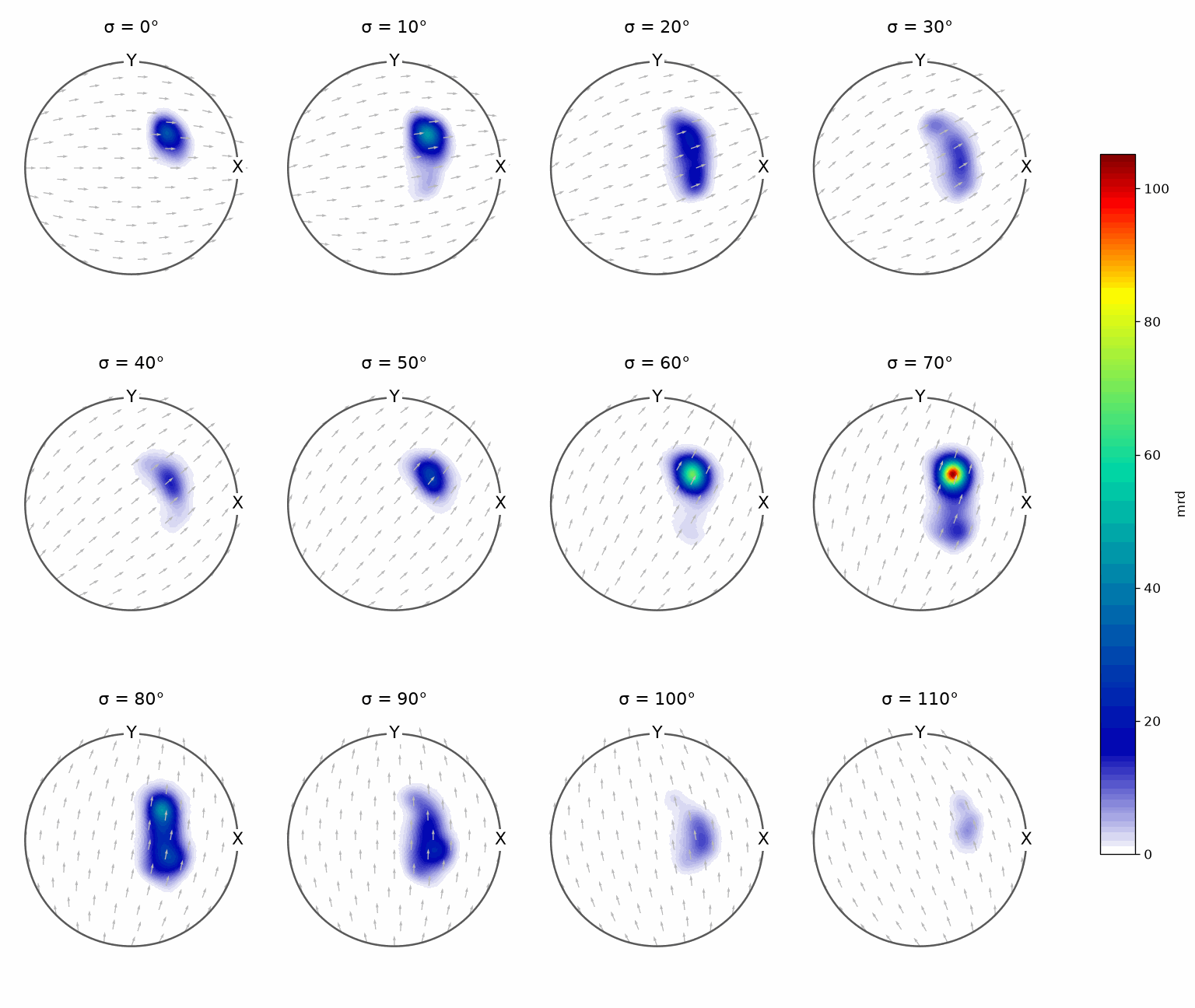
The twelve panels are slices through the same three-dimensional orientation space. Bright compact regions are candidate components, but a feature can continue into a neighbouring slice. Symmetry-equivalent appearances also represent the same physical orientation, not additional components.

The Strongest Mode

A mode is a local maximum of the ODF. The largest mode is the preferred orientation of the whole texture. max returns its density and its orientation.

peakValue, peakOri = max(odf)
peakValue

106.9089

peakOri

orientation (Quartz → y↑→x)
  Bunge Euler angles in degree
  phi1   Phi  phi2
   132  34.6   207

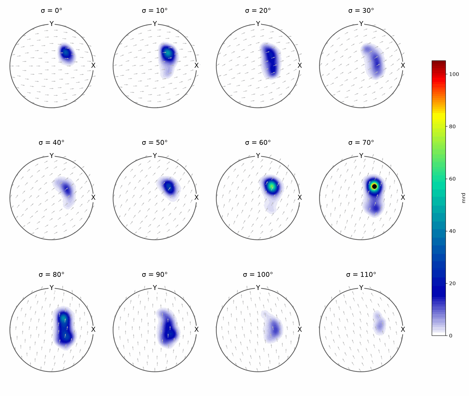
The maximum is 110 multiples of a random distribution (mrd). This is a density, not a percentage of material. The black marker sits in the brightest region of the section plot.

annotate(peakOri, markerFaceColor='black')

Local Modes

With numLocal, max returns the requested number of largest local maxima. Their values are sorted from largest to smallest.

localValue, localOri = max(odf, numLocal=3)
localValue

array([106.9089,  47.7291,  30.3847])

annotate(localOri[1:], markerFaceColor='red')

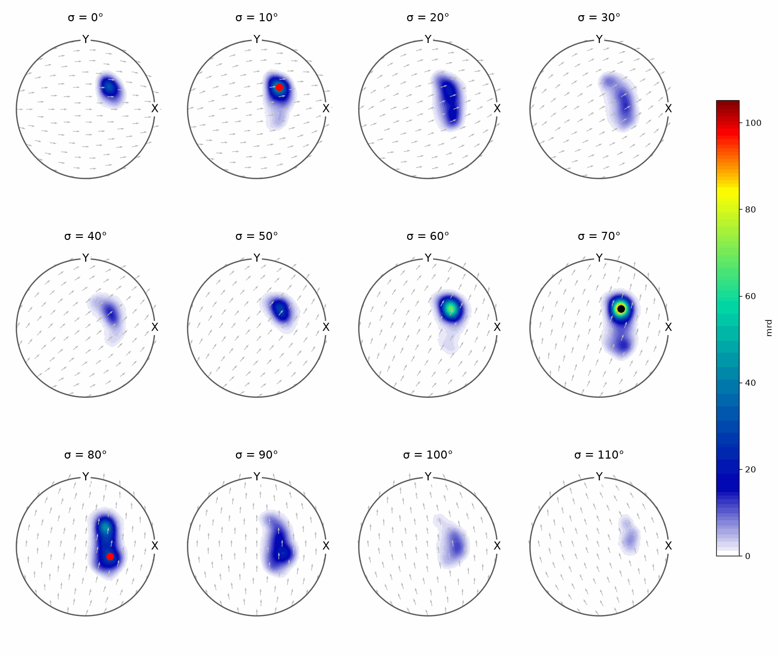
The three modes reach 110, 47, and 32 mrd. The black marker is the global mode and the red markers are the next two. Each lies in a bright neighbourhood; the markers locate peaks but do not define the extent of a component.

These modes belong to the reconstructed ODF, not directly to the measured pole figures. Resolution, kernel halfwidth, and measurement noise can move or merge weak maxima. Check that a small mode persists under reasonable reconstruction or smoothing choices before assigning it to a physical process. ODF Estimation explains those choices.

Volume Inside a Fixed Radius

Peak density is not a measure of component importance. A sharp component can reach a large value while occupying little volume. A reproducible alternative is the fraction of material within a stated disorientation angle of the mode. volume(odf, ori, delta) integrates the ODF over that orientation-space ball.

delta = 10 * degree
ballPercent = 100 * volume(odf, localOri, delta)
ballPercent

array([11.0868,  5.1819,  3.8958])

The three balls contain 11, 5, and 4 percent of the material. Their sum is far below 100 percent because a \(10^\circ\) ball is a small part of orientation space, not because the ODF is missing material. In a uniform texture the same ball would contain

uniformPercent = 100 * volume(uniformODF(odf.CS), localOri[0], delta)
uniformPercent

0.1690

0.17 percent. Dividing by that reference gives the enrichment over a uniform texture.

enrichment = ballPercent / uniformPercent
enrichment

array([65.6124, 30.6667, 23.0558])

The enrichments are 67, 31, and 24. Every value in this section depends on delta. Choosing it too large makes neighbouring balls overlap.

delta = 40 * degree
overlapPercent = 100 * volume(odf, localOri, delta)
overlapPercent

array([58.7376, 34.5041, 43.7729])

overlapTotal = np.sum(overlapPercent)
overlapTotal

137.0146

At \(40^\circ\) the three balls sum to 137 percent. The same orientations are counted in several balls, so the total can exceed 100 percent. These are three separate neighbourhood measurements, not volume fractions of disjoint components.

A Modal Partition

One radius for every component is a strong assumption. Real components need not be spherical, and neighbouring ones can run into each other. calcComponents instead lets seed orientations climb the ODF gradient and groups seeds that reach the same mode.

For this radial-basis ODF, the seeds are its kernel centres and their positive weights. For another representation, MTEX uses an equispaced orientation grid. The shares below are accumulated seed weights. They form a useful modal partition, but they are not integrals over uniquely defined geometric boundaries.

componentOri, componentFraction, _ = calcComponents(odf, verbose=False)
componentPercent = 100 * componentFraction
componentPercent

array([48.4553, 22.0432, 21.8676,  7.6339])

retainedPercent = np.sum(componentPercent)
retainedPercent

100.0000

The four modes contain 48, 22, 21, and 7 percent. They sum to 99 percent because nearly all positive seed weight reaches a retained mode. By default, very small modes may be discarded; use exact=True when retaining them matters.

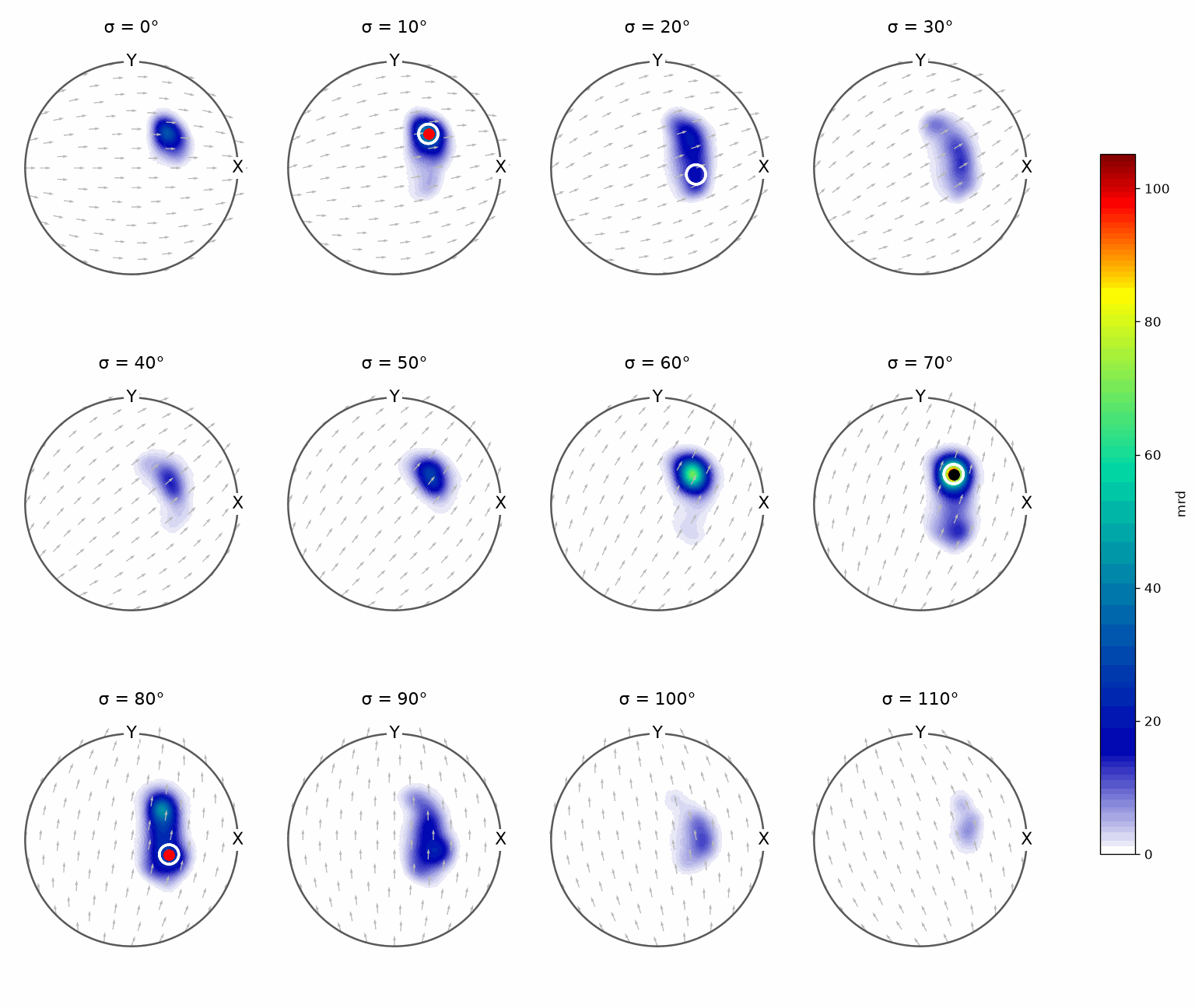
The open white circles show the modal centres. The leading centres agree with the maxima located by max, while the fourth circle appears because the earlier call requested only three local maxima.

annotate(componentOri, markerFaceColor='none', markerEdgeColor='white', lineWidth=2, markerSize=15, marker='o')

Further Reading

• H.-J. Bunge, Texture Analysis in Materials Science, develops the ODF, orientation distance, and symmetry foundations used here.
• U. F. Kocks, C. N. Tomé, and H.-R. Wenk, Texture and Anisotropy, connect preferred orientations and their volume fractions to material anisotropy.
• J.-H. Cho, A. D. Rollett, and K. H. Oh, Determination of Volume Fractions of Texture Components with Standard Distributions in Euler Space, examine component fractions obtained with a misorientation cutoff.
• D. Comaniciu and P. Meer, Mean Shift: A Robust Approach Toward Feature Space Analysis, give the general mode-seeking background for gradient-based density partitions.

Next

Fitting parametric components to an ODF rather than locating them is Modeling. The single numbers that summarise a whole ODF are Properties. Those are global descriptors, whereas the quantities on this page describe selected modes or their neighbourhoods.

Technical Details

max(odf) and max(odf, numLocal=3) return the pair of the values and the orientations, as MATLAB’s two outputs do; localOri[1:] is MATLAB’s localOri(2:end). volume takes a list of orientations and returns one fraction per orientation; calcComponents returns its three outputs, the modes, their weights and the mode of every seed.

@article{bachmann2010mtex,
  author  = {F. Bachmann and R. Hielscher and H. Schaeben},
  title   = {Texture Analysis with MTEX - Free and Open Source Software Toolbox},
  journal = {Solid State Phenomena},
  volume  = {160},
  pages   = {63-68},
  year    = {2010},
  doi     = {10.4028/www.scientific.net/SSP.160.63},
  url     = {https://doi.org/10.4028/www.scientific.net/SSP.160.63}
}