MTEX Scripts

MTEX has no graphical user interface for an analysis. You work with MTEX by writing Python scripts: text files that keep the commands for an analysis in a reproducible order.

A typical script follows five steps.

1. Import data.
2. Inspect the imported data.
3. Correct the data when necessary.
4. Analyze the data.
5. Plot and export the results.

During these steps, Python stores data under names called variables. Each variable has a type, called its class, which determines the operations that can be applied to it. MTEX provides classes for objects such as vectors, rotations, EBSD data, grains, and orientation distribution functions (ODFs). The Function Reference lists all MTEX classes and functions.

from mtex import *

Import and inspect data

Import functions create variables automatically. Here, fileName stores the path to an example CTF file. The second command imports that file and stores the result in the variable ebsd.

fileName = mtexdatafile('forsterite')
ebsd = EBSD.load(fileName, eulerCorrection=rotation.byAxisAngle(xvector, 180 * degree))
ebsd

EBSD (y↓→x)
  size: 336 × 732 grid
  Phase  Orientations  Mineral     Color         Symmetry  Crystal reference frame
  0      58485 (24%)   notIndexed
  1      152345 (62%)  Forsterite  LightSkyBlue  mmm       Forsterite
  2      26058 (11%)   Enstatite   DarkSeaGreen  mmm       Enstatite
  3      9064 (3.7%)   Diopside    Goldenrod     12/m1     Diopside
  properties    : bands, bc, bs, error, mad
  scan unit     : um
  X × Y         : [0 → 3.655e+04] × [0 → 1.675e+04]
  square lattice: spacing 50

Writing the variable’s name on its own line displays a summary of ebsd. This is a quick inspection step: the summary reports the phases, numbers of orientations, properties, map extent, and grid size. The eulerCorrection option also corrects the imported orientations by the specified rotation.

Plot the phase map

Pass a variable to an MTEX function to operate on its data. The command below passes ebsd to plot and colors every indexed measurement by its phase.

plot(ebsd)

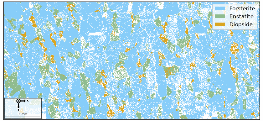
Notice the large blue forsterite regions, the smaller green enstatite and yellow diopside regions, and the white notIndexed areas. A notIndexed measurement is one whose diffraction pattern could not be indexed.

Reconstruct and inspect grains

The next command segments the measurements into grains. A grain is a phase-homogeneous, spatially connected region of EBSD measurements produced by segmentation. The minPixel option excludes indexed grains with fewer than three measurements.

grains = calcGrains(ebsd, minPixel=3)
grains

grain2d (y↓→x)
  size: 962
  Phase  Grains               Mineral     Color         Symmetry  Crystal reference frame
  0      19 (1306 pixels)     notIndexed
  1      490 (151673 pixels)  Forsterite  LightSkyBlue  mmm       Forsterite
  2      224 (25736 pixels)   Enstatite   DarkSeaGreen  mmm       Enstatite
  3      229 (7673 pixels)    Diopside    Goldenrod     12/m1     Diopside
  boundary segments: 36604, inner: 282, triple points: 1579

The returned grain2d object is stored in grains. Its summary reports the number of grains in each phase and information about their boundaries.

Add the grain boundaries

Plotting on the same axes connects the result of the analysis to the phase map. hold(True) preserves the existing map while the boundary is added, and hold(False) ends that plotting state.

hold(True)
plot(grains.boundary, lineWidth=2)
hold(False)

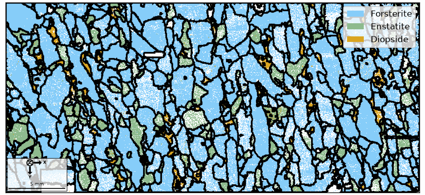
Notice that the dark lines trace changes between neighboring grains. Some lines lie within one color because grains of the same phase can still have different orientations.

Organize a script

An MTEX script is a sequence of Python and MTEX commands. Add comments on lines beginning with # to record why each command is present. These explanations make the analysis understandable when the script is reopened.

Divide a longer script into cells with lines beginning with # %%. In VS Code, Spyder or PyCharm, Shift+Enter runs the current cell in an interactive window and advances to the next one. Running one cell at a time lets you inspect each intermediate variable before continuing. A Jupyter notebook is the same sequence of cells in another file format; jupytext converts between the two, and every page of this documentation is such a script (docs/notebook.py <Page> opens one as a notebook).

References

• Python Software Foundation, The Python Tutorial, Python documentation, and Microsoft, Python Interactive window, VS Code documentation. They explain script files, comments, and the cells used on this page. The MATLAB page cites MathWorks’ Create Scripts.

Next

Continue with Lists and Indexing to select parts of an MTEX variable and apply one operation to many stored objects.

@article{bachmann2010mtex,
  author  = {F. Bachmann and R. Hielscher and H. Schaeben},
  title   = {Texture Analysis with MTEX - Free and Open Source Software Toolbox},
  journal = {Solid State Phenomena},
  volume  = {160},
  pages   = {63-68},
  year    = {2010},
  doi     = {10.4028/www.scientific.net/SSP.160.63},
  url     = {https://doi.org/10.4028/www.scientific.net/SSP.160.63}
}