A method of EBSD.

the measurements along a polyline, in the order they are met, and the distance along the line of each of them; MATLAB’s spatialProfile

Syntax

ebsdLine, dist = spatialProfile(ebsd, [15.5, 27], [20.5, 11])

One segment, x and y.

ebsdLine, dist = spatialProfile(ebsd, xy)

A polyline, (N, 2) points.

ebsdLine, dist = spatialProfile(ebsd, xy, radius=1)

A wider band.

Description

A pixel belongs to the line when it lies within radius of one of its segments, half a step by default; a pixel at the joint of two segments is met once.

Input

`ebsd`	EBSD
`lineXY`	(N, 2) array of the points of the line, or their x coordinates
`y`	the y coordinates, when lineXY gives x

Keywords

keyword	default	description
`radius`	`None`	the half width of the band around the line, in the scan unit

Output

`ebsdLine`	EBSD, the measurements along the line
`dist`	array, the distance of each along the line from its first point

Example

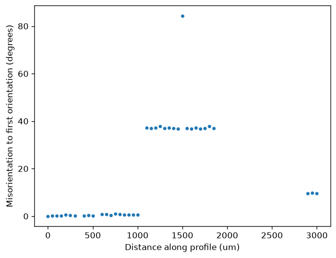
Extract a horizontal profile through the small Forsterite map and plot its misorientation relative to the first selected orientation. The sample is cached after its first download.

import numpy as np
import matplotlib.pyplot as plt
from mtex import mtexdata, spatialProfile, degree

ebsd = mtexdata('small', verbose=False)['Forsterite']
y = float(np.median(ebsd.y))
line = [[float(np.min(ebsd.x)), y], [float(np.max(ebsd.x)), y]]
profile, distance = spatialProfile(ebsd, line)
omega = profile.orientations.angle(profile.orientations[0])/degree
print('Selected measurements:', profile.size)
print('Distance increases:', bool(np.all(np.diff(distance) >= 0)))
plt.plot(distance, omega, '.')
plt.xlabel('Distance along profile (um)')
plt.ylabel('Misorientation to first orientation (degrees)')
plt.show()

Distances use the scan unit and start at the first line endpoint. The default band extends half a lattice step on either side of the line; radius changes that band. Large jumps can mark different grains. This extracts measured pixels rather than interpolating an orientation field.

Selected measurements: 38
Distance increases: True

Example output for EBSD.spatialProfile

Citing this page. This page is part of the documentation of MTEX, a free and open source MATLAB toolbox for analyzing and modeling crystallographic textures. It was written by The MTEX Developers and is published at https://mtex-toolbox.github.io/EBSDsquare.spatialProfile_py.html. If you use MTEX, or reuse text or figures from this page, in your research, please cite

F. Bachmann, R. Hielscher, H. Schaeben: Texture Analysis with MTEX - Free and Open Source Software Toolbox, Solid State Phenomena 160 (2010), 63-68. 10.4028/www.scientific.net/SSP.160.63

BibTeX

@article{bachmann2010mtex,
  author  = {F. Bachmann and R. Hielscher and H. Schaeben},
  title   = {Texture Analysis with MTEX - Free and Open Source Software Toolbox},
  journal = {Solid State Phenomena},
  volume  = {160},
  pages   = {63-68},
  year    = {2010},
  doi     = {10.4028/www.scientific.net/SSP.160.63},
  url     = {https://doi.org/10.4028/www.scientific.net/SSP.160.63}
}

Other papers describing specific MTEX methods are listed under Publications — please cite the one that best fits your application. The MTEX source code is licensed under the GNU General Public License v2.0; the text and figures of this documentation are licensed under CC BY 4.0, which permits reuse — including by automated systems — provided The MTEX Developers and this page are credited.

EBSDsquare.spatialProfile