download as script · edit page

Many scientific figures put related information together. Examples include measurements over a fitted function, two data sets in one projection, or crystal directions on an inverse pole figure.

MTEX offers three ways to combine plots. The right choice depends on whether the figure has one axis, several managed axes, or independent panels.

This page assumes the plot types from Plot Types and the screen frame from Axes Alignment. The examples also use pole figures, inverse pole figures, and three-dimensional orientation plots. Follow the links where each first appears if these are unfamiliar.

import matplotlib.pyplot as plt

from mtex import *

plottingConvention.default('y↑→x')

Holding a Plot

The MATLAB way is hold on, here hold(True). It keeps what is drawn, so the next command adds to it rather than replacing it. The command hold(False) ends that state.

plt.close('all')
plt.plot([1, 2], [2, 2], linewidth=2)

hold(True)

plt.plot([1, 2], [1, 3], linewidth=2)

hold(False)

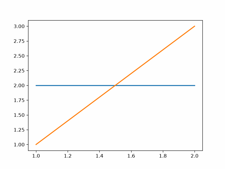
The sloping line is added without erasing the horizontal one. After hold(False), the next high-level plotting command may replace both.

Two Data Sets in One Projection

Start with a compact set of orientations and rotate a copy of its parent distribution.

cs = crystalFrame('-3m')
odf = unimodalODF(orientation.byEuler(0, 0, 0, cs))
ori = discreteSample(odf, 100)
oriRotated = discreteSample(rotate(odf, rotation.byEuler(60 * degree, 60 * degree, 0 * degree)), 100)

Draw both sets in axis–angle space. Each orientation becomes a point whose direction is its rotation axis. Its distance from the origin is the rotation angle. See 3D Orientation Visualizations for this representation.

scatter(ori, 'axisAngle')
hold(True)   # keep plot
scatter(oriRotated)
hold(False)  # next plot command deletes all plots

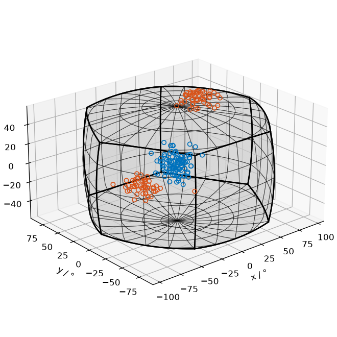
The figure holds three clouds. The original set is a single compact blob near the origin. The rotated set is one cluster too, but it appears as two lobes in opposite corners of the region: once a cluster sits far from the identity, its symmetrically equivalent representatives no longer all fall in the same corner.

Either way the rotated points occupy different ground from the original ones, which shows that the rotation changed the orientations rather than only their plotted description.

The Same Data in Pole Figures

Project the same comparison along two crystal directions. The second plotPF does not repeat the antipodal flag. The existing axes already define that symmetry. Added data must conform to those axes.

h = [Miller(0, 0, 0, 1, cs), Miller(1, 0, -1, 0, cs)]
plotPF(ori, h, antipodal=True, markerSize=4)
hold(True)
plotPF(oriRotated, h, markerSize=4)
hold(False)

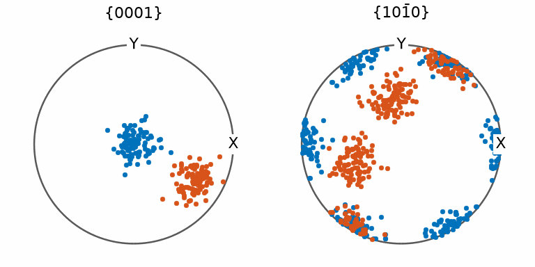
Both pole-figure panels contain the two orientation sets. Here plotPF sees the two crystal directions. It adds the second set to both matching axes. That multi-axis behaviour belongs to plotPF, not to hold itself.

Adding to Every Axis at Once

hold(True) changes only the current axis. A pole-figure figure has one axis per crystal direction. The general way to add one data set to every MTEX axis is the add2all flag.

plotPF(odf, h, antipodal=True, contourf=True, grid=True)
mtexColorMap('white2black')

plot(ori, displayName='original', markerSize=5, markerFaceColor='b', markerEdgeColor='w', add2all=True)

plot(oriRotated, displayName='rotated', markerSize=5, markerFaceColor='r', markerEdgeColor='k', add2all=True)

legend('show', location='northeast')

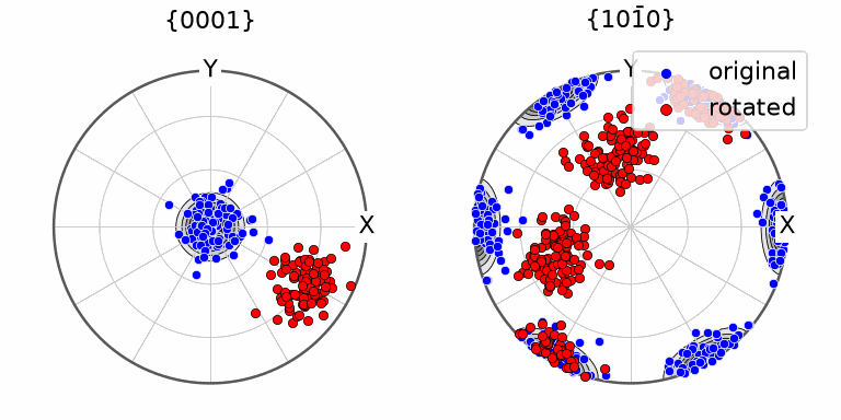
Each orientation set appears in both pole figures after one command. MTEX reprojects the orientations according to the crystal direction stored on each axis. Plain hold(True) neither selects all axes nor performs that dispatch.

ODF sections work the same way, and here it matters more: there are eight axes, and every orientation belongs in the section closest to it.

plotSection(odf, 'sigma', sections=8, contourf=True)
mtexColorMap('white2black')
plot(ori, markerSize=6, markerFaceColor='b', markerEdgeColor='w', add2all=True)
plot(oriRotated, markerSize=6, markerFaceColor='r', markerEdgeColor='k', add2all=True)

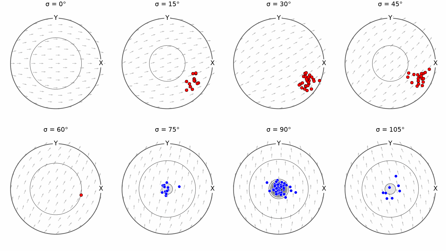
Both sets place markers in every section, so the section a marker lands in does not by itself separate the two. What distinguishes them is where they sit within a section: the original markers follow the contours of the ODF, and the rotated ones do not.

Marking Crystal Directions

An inverse pole figure fixes a specimen direction and maps the crystal directions parallel to it. See Inverse Pole Figures for the construction. Marking important crystal directions makes the plot readable. The symmetrised flag draws every symmetrically equivalent direction, while labeled writes the indices beside them.

plotIPF(odf, xvector, axisLabels=False)
mtexColorMap('white2black')

hold(True)   # keep plot
plot(Miller(0, 0, 0, 1, cs), symmetrised=True, labeled=True, backgroundColor='w')
plot(Miller(1, 1, -2, 0, cs), symmetrised=True, labeled=True, backgroundColor='w')
plot(Miller(0, 1, -1, 0, cs), symmetrised=True, labeled=True, backgroundColor='w')
plot(Miller(0, 1, -1, 1, cs), symmetrised=True, labeled=True, backgroundColor='w')
hold(False)  # next plot command deletes all plots

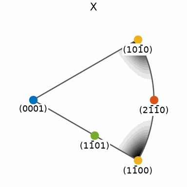
The labels expose an important correction: the maximum is not at (0001). This ODF is centred on the identity orientation, so specimen X corresponds to a crystal direction in the basal plane. A c-axis maximum would instead appear in the inverse pole figure for specimen Z.

Different Plots Side by Side

The third case arranges several independent plots rather than overlaying them. The MTEX commands used below accept a parent axes, so matplotlib’s own subplot can do the arranging.

pf = mtexdata('dubna')

odf = calcODF(pf, verbose=False)

A measured, a recalculated, and a difference pole figure form the standard comparison for judging a reconstruction. See ODF Estimation for the reconstruction workflow.

plt.figure(figsize=(12, 5))

# set position 1 in a 1x3 matrix as the current plotting position
axesPos = plt.subplot(1, 3, 1)

# plot pole figure 1 at this position
plot(pf[0], parent=axesPos)

# set position 2 in a 1x3 matrix as the current plotting position
axesPos = plt.subplot(1, 3, 2)

# plot the recalculated pole figure at this position
plotPF(odf, pf.allH[0], antipodal=True, parent=axesPos)

# set position 3 in a 1x3 matrix as the current plotting position
axesPos = plt.subplot(1, 3, 3)

# plot the difference pole figure at this position
plotDiff(odf, pf[0], parent=axesPos)

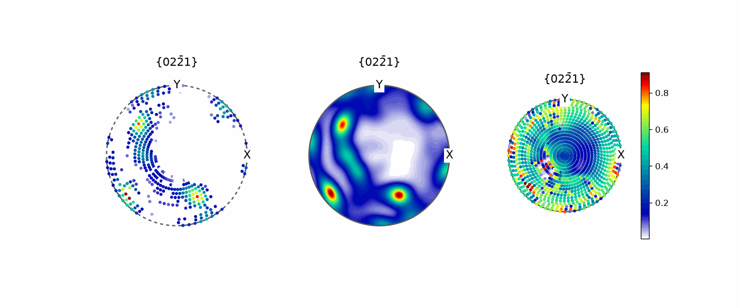
From left to right, the panels show the measured intensity, the smoother intensity recalculated from the ODF, and their relative difference. The last panel locates mismatches that the first two panels make hard to judge. Compare colour values only when the relevant panels use the same range.

Combined Plots