Inverse Pole Figures of an ODF

A pole figure fixes a crystal direction and asks where it points in the specimen. An inverse pole figure fixes a specimen direction \(\vec r\) and asks which crystal directions \(\vec h\) point along it.

This page assumes the ODF and multiples-of-a-random-distribution (mrd) normalization from ODF Theory. Crystal directions are introduced in Crystal Directions. The projection itself is introduced in Spherical Projections. Inverse Pole Figures builds the same construction first for individual orientations rather than an ODF.

Formally, the inverse pole density is the ODF integrated along every orientation that maps \(\vec h\) onto \(\vec r\),

These orientations form an orientation fibre. The plot therefore loses the rotation about the aligned direction. Here inverse means that the specimen and crystal directions exchange roles; it does not mean reconstructing or numerically inverting the ODF.

The result is a density in mrd, not a percentage at one point. Inverse pole figures are natural when one specimen direction carries the physical question: a sheet normal, a compression axis, or an EBSD map surface normal.

A plotting convention states how a reference frame is laid out on screen. The following convention draws specimen Y upward and specimen X to the right. It does not rotate the specimen or change the ODF.

import numpy as np

from mtex import *

plottingConvention.default('y↑→x')

A Model Texture to Look At

This is the same three-component texture as on the pole-figure page. It combines two localized components with a fibre component that aligns the crystal c-axis with specimen X.

cs = crystalFrame('32')
mod1 = orientation.byEuler(90 * degree, 40 * degree, 110 * degree, 'ZYZ', cs)
mod2 = orientation.byEuler(50 * degree, 30 * degree, -30 * degree, 'ZYZ', cs)

odf = 0.2 * unimodalODF(mod1) + 0.3 * unimodalODF(mod2) + 0.5 * fibreODF(Miller(0, 0, 1, cs), vector3d.X, halfwidth=10 * degree)

# convert once so repeated Radon transforms reuse Fourier coefficients
odf = SO3FunHarmonic(odf, bandwidth=32)

Plotting Specimen Directions

plotIPF works like plotPF, except that its input directions belong to the specimen frame. The coordinates inside each panel are crystal directions. This frame reversal is the point of an inverse pole figure.

plotIPF(odf, cat(vector3d.X, vector3d.Z))
mtexColorMap('LaboTeX')
mtexColorbar(title='mrd')

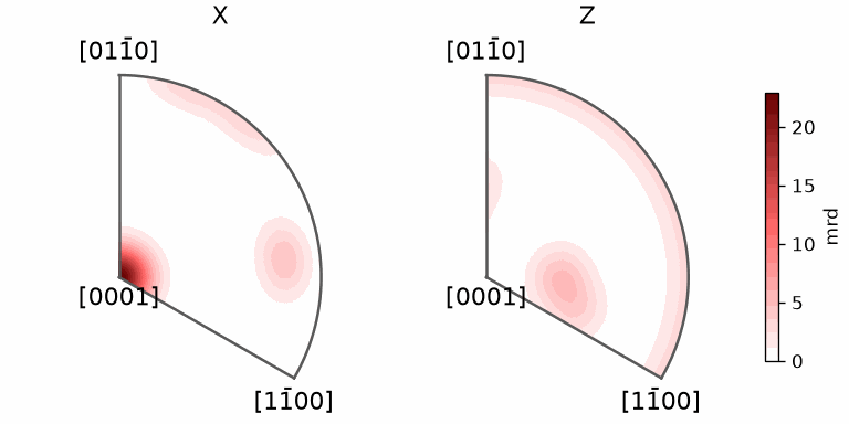
The fibre component puts the c-axis along X, so the \((0001)\) corner is the maximum of the X inverse pole figure. The same corner is almost empty for Z. One inverse pole figure still does not determine full orientations, because every value collects an entire orientation fibre.

Values Rather Than Colours

radon with only a specimen direction, r=, returns an inverse pole density function. Its printed summary identifies the returned spherical-function representation and crystal symmetry.

ipdfX = radon(odf, r=vector3d.X)
ipdfZ = radon(odf, r=vector3d.Z)
ipdfX

S2FunHarmonic (321)
  bandwidth: 25
  mean     : 1

densitySummary = np.array([[ipdfX.eval(cs.cAxis), ipdfZ.eval(cs.cAxis)], [max(ipdfX)[0], max(ipdfZ)[0]]])
densitySummary

array([[22.9594,  0.0249],
       [22.9594,  5.4244]])

The first row is the density at \((0001)\): about 23 mrd for X and 0.021 mrd for Z. The second row contains the maxima. For X the c-axis corner is itself the maximum; for Z the maximum is about 5.2 mrd elsewhere in the sector. An inverse pole figure answers which crystal direction prefers one chosen specimen direction.

Antipodal Symmetry

The antipodal flag identifies a crystal direction with its opposite. It replaces \(P_{\vec r}(\vec h)\) by the average of its values at \(\vec h\) and \(-\vec h\). This halves the region that has to be drawn, exactly as for axes. This is a modelling choice, not a display option. Use it only when the measurement or model cannot distinguish the directions.

plotIPF(odf, cat(vector3d.X, vector3d.Z), antipodal=True)
mtexColorMap('LaboTeX')

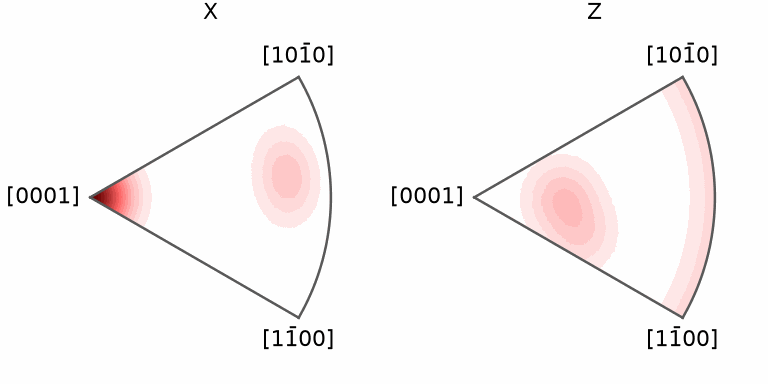
Notice both changes: the sector is smaller, and its colours can differ because opposite-direction densities have been averaged.

The Complete Sphere

By default MTEX draws only the fundamental sector. Every point outside it is a symmetry-equivalent copy of one inside. The complete flag expands those copies, while upper retains only the upper hemisphere. Neither flag changes the density.

plotIPF(odf, cat(vector3d.X, vector3d.Z), complete=True, upper=True)
mtexColorMap('LaboTeX')

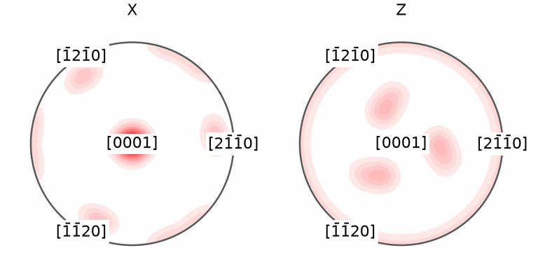
The threefold symmetry of point group 32 is now visible as three repeats around the c-axis. They are symmetry-equivalent appearances of the same texture features, not three additional components.

Separating Symmetrization from the Displayed Region

Keep the same complete upper hemisphere and impose antipodal symmetry. This isolates the change in density from the change in plotted region.

plotIPF(odf, cat(vector3d.X, vector3d.Z), complete=True, antipodal=True, upper=True)
mtexColorMap('LaboTeX')

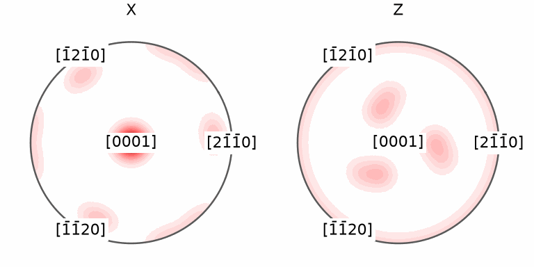
The X plot gains three faint rim lobes from directions whose opposites were in the lower hemisphere. The localized Z lobes become broader averaged features. These changes come from the antipodal average, not from displaying a different part of the sphere.

An inverse pole density of an ODF is not an EBSD colour key. A colour key assigns colours to the same crystal-direction sector but does not itself show how much material lies there.

Further Reading

• H.-J. Bunge, Texture Analysis in Materials Science: Mathematical Methods, Butterworths, 1982. It develops pole figures, inverse pole figures, and ODFs together.
• D. Chateigner, L. Lutterotti, and M. Morales, Quantitative texture analysis and combined analysis, International Tables for Crystallography H, ch. 5.3, 2019. It defines inverse pole densities and illustrates the symmetry-reduced sectors.
• ASTM International, ASTM E81-96(2024): Standard Test Method for Preparing Quantitative Pole Figures. It distinguishes measured pole figures from calculated pole and inverse pole figures.

Next

Colouring an EBSD map by where each orientation falls in this sector is IPF Maps. The other projection is Pole Figures. Continue to the unprojected slices in Euler Angle Sections and Sigma Sections. If the ODF must first be reconstructed from diffraction data, continue to ODF Reconstruction.

Technical Details

MATLAB’s empty crystal direction [] is None here: calcPDF(odf, None, r) returns the inverse pole density function. max(ipdf) returns the pair of the value and the direction, so the summary takes its first element.

@article{bachmann2010mtex,
  author  = {F. Bachmann and R. Hielscher and H. Schaeben},
  title   = {Texture Analysis with MTEX - Free and Open Source Software Toolbox},
  journal = {Solid State Phenomena},
  volume  = {160},
  pages   = {63-68},
  year    = {2010},
  doi     = {10.4028/www.scientific.net/SSP.160.63},
  url     = {https://doi.org/10.4028/www.scientific.net/SSP.160.63}
}