
Texture and microstructure analysis
Analyse 2D and 3D EBSD maps, pole figures and orientations in MATLAB or Python. Every analysis step is a few lines of code.
Unzip and run startup_mtex in MATLAB R2022b or newer.
What is newAll releasesSpeed of the versionsSource on GitHub
MTEX for Python 1.0 · Python 3.12+ · no MATLAB licence needed.
 Import your own dataThe import wizard reads your file and writes the script that loads it.
Then follow the EBSD tutorial →
Import your own dataThe import wizard reads your file and writes the script that loads it.
Then follow the EBSD tutorial →


You are not on your own. Ask in the forum with 1,400 discussions, build on code of 43 contributors, and meet us at the workshop every year.
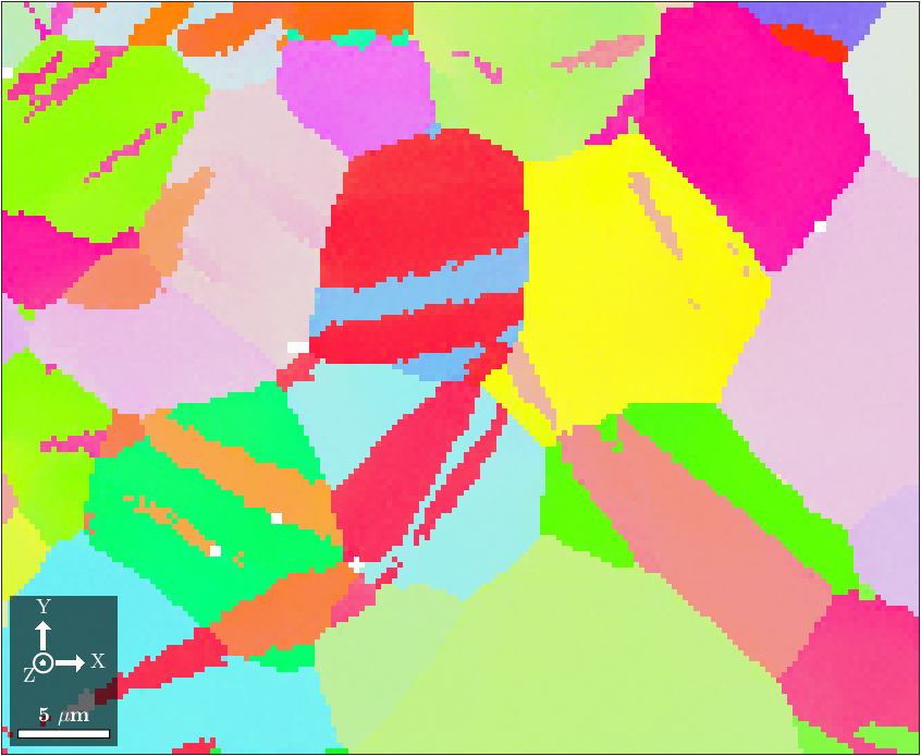
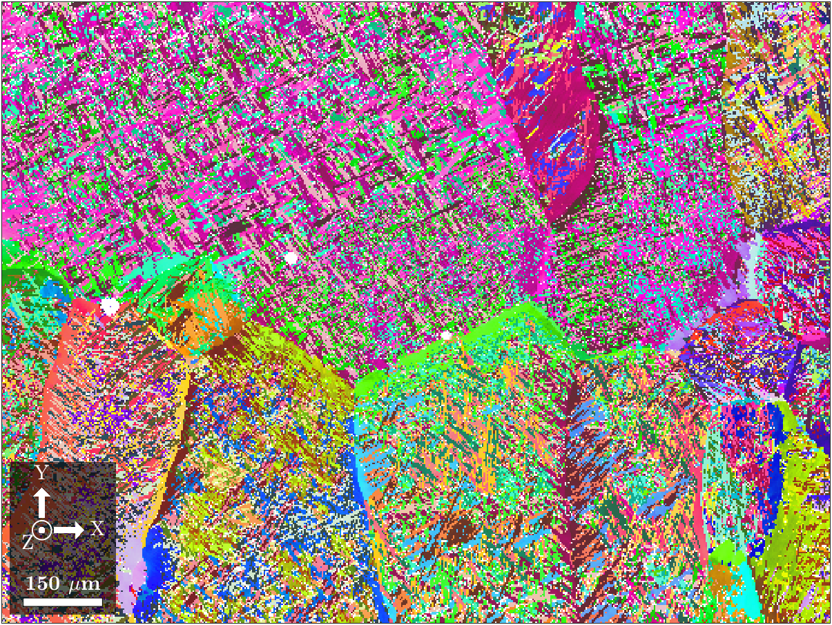
% load a magnesium EBSD map
ebsd = EBSD.load('twins.h5');

plot(ebsd('Magnesium'),'ipfDirection',zvector)
# load a magnesium EBSD map
ebsd = EBSD.load('twins.h5')

plot(ebsd['Magnesium'],ipfDirection=zvector)
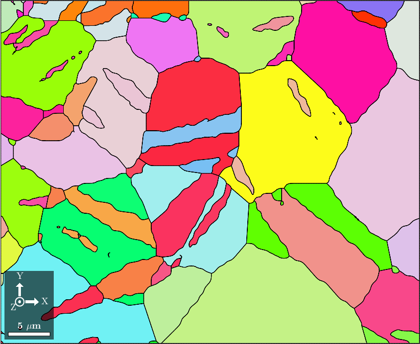
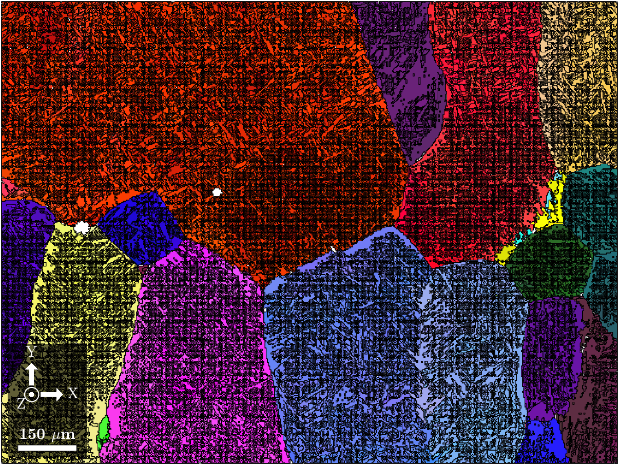
% reconstruct grains and smooth boundaries
[grains,ebsd] = calcGrains(ebsd,'angle',5*degree);
grains = smoothBoundary(grains,5);
plot(grains,'ipfDirection',zvector)
# reconstruct grains and smooth boundaries
grains = calcGrains(ebsd,angle=5*degree)
grains = smoothBoundary(grains,5)
plot(grains,ipfDirection=zvector)
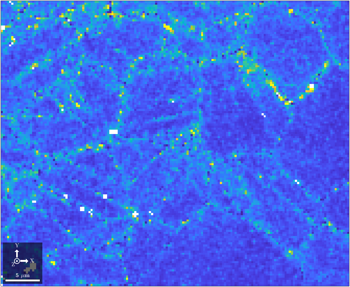
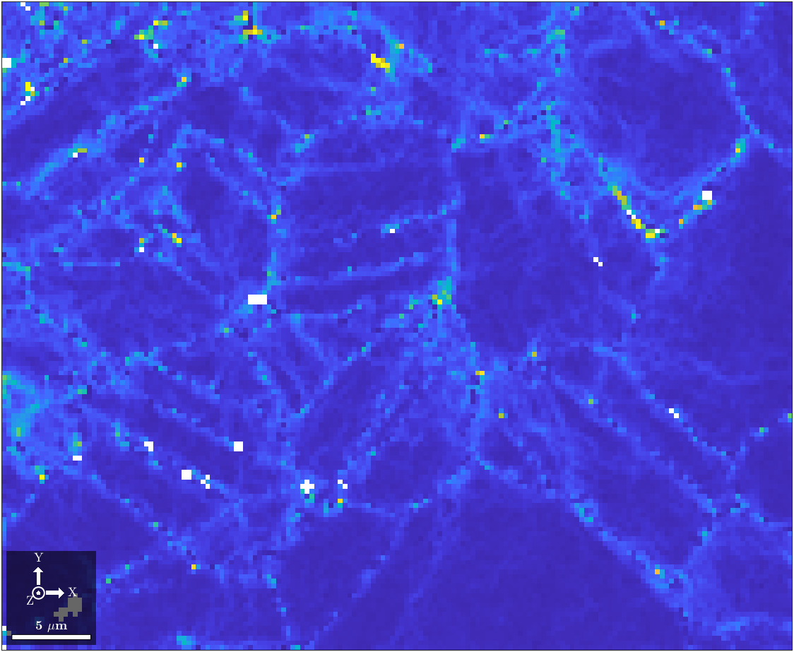
% denoise the orientations
ebsdS = smooth(ebsd,l1TVFilter);

% compare kernel average misorientation
plot(ebsd,ebsd.KAM./degree)
plot(ebsdS,ebsdS.KAM./degree)
# denoise the orientations
ebsdS = smooth(ebsd,l1TVFilter())

# compare kernel average misorientation
plot(ebsd,ebsd.KAM()/degree)
plot(ebsdS,ebsdS.KAM()/degree)
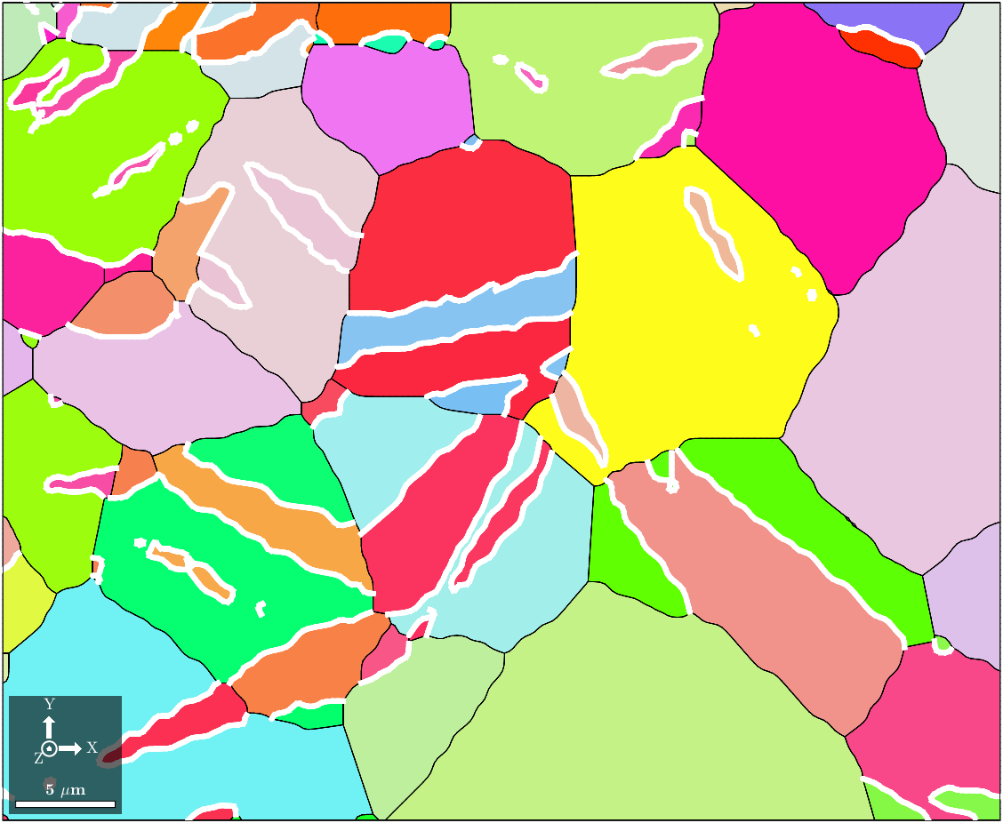
% magnesium {10-12} extension twin
twin = orientation.byAxisAngle(...
  Miller(1,0,-1,2,grains.CS),180*degree);
gB = grains.boundary('Magnesium','Magnesium');
twinB = gB(gB.isTwinning(twin,5*degree));
plot(twinB,'lineColor','w','lineWidth',3)

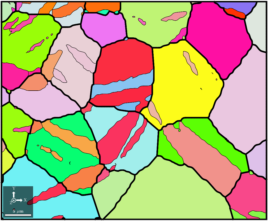
% merge grains across twin boundaries
parents = merge(grains,twinB);
plot(parents.boundary,'lineWidth',3)
# magnesium {10-12} extension twin
twin = orientation.byAxisAngle(
  Miller(1,0,-1,2,grains.CS),180*degree)
gB = grains.boundary['Magnesium','Magnesium']
twinB = gB[gB.isTwinning(twin,5*degree)]
plot(twinB,lineColor='w',lineWidth=3)

# merge grains across twin boundaries
parents = merge(grains,twinB)
plot(parents.boundary,lineWidth=3)
% estimate the orientation distribution
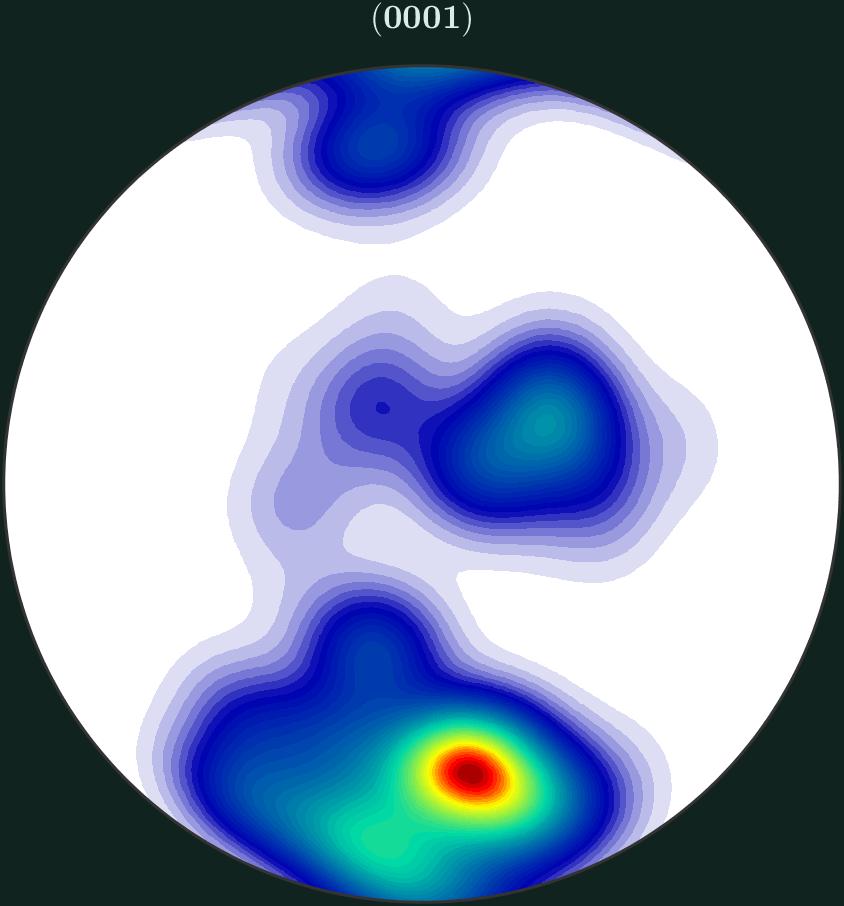
odf = calcDensity(ebsd('Magnesium').orientations,...
  'halfwidth',10*degree);

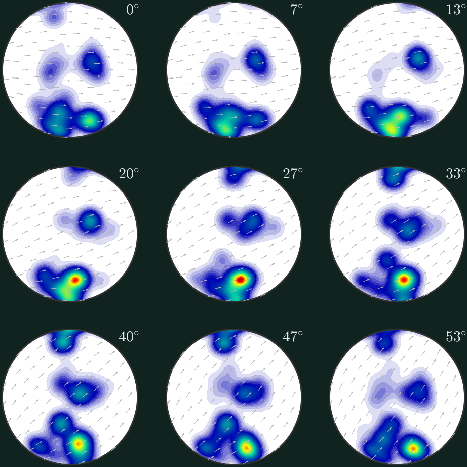
% show a pole figure and ODF sections
plotPDF(odf,Miller(0,0,0,1,odf.CS))
plotSection(odf,'sigma','sections',9)
# estimate the orientation distribution
odf = calcDensity(ebsd['Magnesium'].orientations,
  halfwidth=10*degree)

# show a pole figure and ODF sections
plotPF(odf,Miller(0,0,0,1,odf.CS))
plotSection(odf,'sigma',sections=9)
% reconstruct beta grains from alpha titanium
mtexdata alphaBetaTitanium
job = parentGrainReconstructor(ebsd);
job.p2c = orientation.Burgers(job.csParent,job.csChild);

% group variants and assign parent orientations
job.calcVariantGraph('threshold',1.5*degree);
job.clusterVariantGraph('numIter',3);
job.calcParentFromVote;
plot(job.parentGrains,'ipfDirection',zvector)
# reconstruct beta grains from alpha titanium
ebsd = mtexdata('alphaBetaTitanium')
job = parentGrainReconstructor(ebsd)
job.p2c = orientation.Burgers(job.csParent,job.csChild)

# group variants and assign parent orientations
job.calcVariantGraph(threshold=1.5*degree)
job.clusterVariantGraph(numIter=3)
job.calcParentFromVote()
plot(job.parentGrains,ipfDirection=zvector)
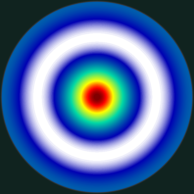
% single-crystal stiffness of magnesium (GPa)
Cij = [59.7 26.2 21.7 0 0 0;  26.2 59.7 21.7 0 0 0;
       21.7 21.7 61.7 0 0 0;  0 0 0 16.4 0 0;
       0 0 0 0 16.4 0;  0 0 0 0 0 16.75];
C = stiffnessTensor(Cij,ebsd('Magnesium').CS);

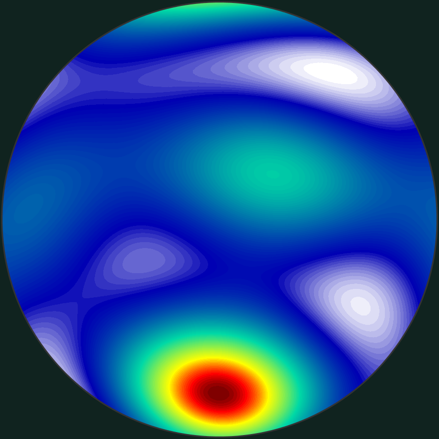
% average over the measured texture (Hill)
[~,~,CHill] = calcTensor(ebsd('Magnesium'),C);
plot(C.YoungsModulus,'complete','upper')
plot(CHill.YoungsModulus,'complete','upper')
# single-crystal stiffness of magnesium (GPa)
Cij = [[59.7,26.2,21.7,0,0,0], [26.2,59.7,21.7,0,0,0],
       [21.7,21.7,61.7,0,0,0], [0,0,0,16.4,0,0],
       [0,0,0,0,16.4,0], [0,0,0,0,0,16.75]]
C = stiffnessTensor(Cij,ebsd['Magnesium'].CS)

# average over the measured texture (Hill)
CHill = calcTensor(ebsd['Magnesium'],C,'Hill')
plot(C.YoungsModulus(),complete=True,upper=True)
plot(CHill.YoungsModulus(),complete=True,upper=True)
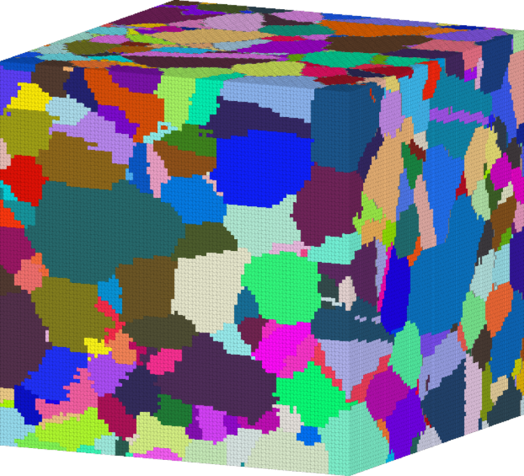
% a 3D EBSD volume and its grains
fname = fullfile(mtexEBSDPath,'SmallIN100_MeshStats.dream3d');
ebsd = EBSD3.load(fname);
[grains,ebsd] = calcGrains(ebsd,'angle',5*degree);
plot(grains,grains.meanOrientation,'edgeAlpha',0.1)

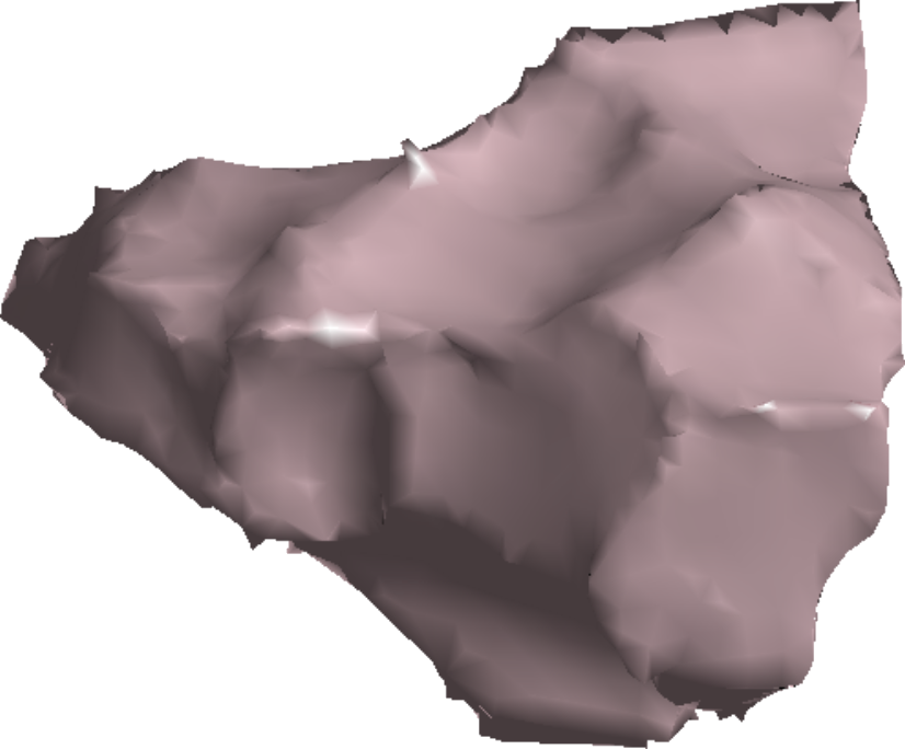
[~,id] = max(grains.volume);
grains = reduceBoundary(grains,2,'quadric');
grains = smoothBoundary(grains,taubinFilter(20));
plot(grains(id),grains(id).meanOrientation,'edgeAlpha',0)
camlight; lighting gouraud
# a 3D EBSD volume and its grains
ebsd = EBSD3.load(mtexdatafile('SmallIN100'))
grains = calcGrains(ebsd,angle=5*degree)
plot(grains,grains.meanOrientation,edgeAlpha=0.1)

id = grains.volume.argmax()
plot(grains[id],grains[id].meanOrientation,edgeAlpha=0.2)
What MTEX gives you
Read data from any source
Whatever the instrument, the data lands in one data model and runs through the same algorithms, so maps from different microscopes compare directly.
Beyond the acquisition software
MTEX goes on where acquisition software stops: it covers analyses the vendors leave out and brings diffraction and EBSD data together in one place.
Open, down to the algorithm
No black box: every function is source code you can open, and every parameter is yours to set. The core algorithms are published in peer-reviewed papers.
Workshop on Quantitative Microstructure Analysis
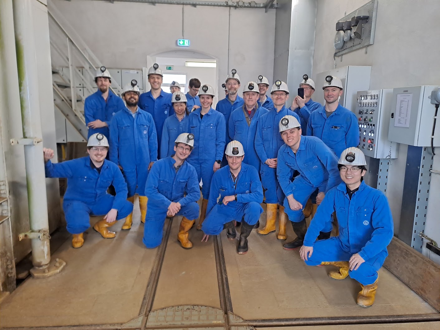
Two weeks with the MTEX developers. The first week teaches texture and microstructure analysis from the ground up. In the second you bring your own data and work on it with experts from metallurgy, geology and semiconductors.
Programme and registrationAI assistants write MTEX scripts you can check
Describe your analysis in plain words and an assistant drafts the script. The documentation is mapped for AI tools in llms.txt. The result is ordinary code, so you read it, run it and keep it with your data.
I have an Oxford map A.ctf and an EDAX map B.ang of the same single-phase steel. Compare the grain size distributions.
% two vendors, one grain definition
ebsdA = EBSD.load('A.ctf');
ebsdB = EBSD.load('B.ang');
grainsA = calcGrains(ebsdA,'angle',10*degree);
grainsB = calcGrains(ebsdB,'angle',10*degree);

% shared bins, normalized for different map sizes
rA = grainsA('indexed').equivalentRadius;
rB = grainsB('indexed').equivalentRadius;
edges = linspace(0,max([rA(:);rB(:)]),21);
histogram(rA,edges,'Normalization','pdf',...
  'DisplayStyle','stairs')
hold on
histogram(rB,edges,'Normalization','pdf',...
  'DisplayStyle','stairs')
hold off
xlabel('Equivalent radius (map length units)')
ylabel('Probability density')
legend('Oxford','EDAX')
import numpy as np
# two vendors, one grain definition
ebsdA = EBSD.load('A.ctf')
ebsdB = EBSD.load('B.ang')
grainsA = calcGrains(ebsdA,angle=10*degree)
grainsB = calcGrains(ebsdB,angle=10*degree)

# shared bins, normalized for different map sizes
rA = grainsA['indexed'].equivalentRadius
rB = grainsB['indexed'].equivalentRadius
edges = np.linspace(0,max(rA.max(),rB.max()),21)
histogram(rA,edges,density=True,histtype='step',label='Oxford')
hold(True)
histogram(rB,edges,density=True,histtype='step',label='EDAX')
hold(False)
xlabel('Equivalent radius (map length units)')
ylabel('Probability density')
legend()