selectHalfwidth

Select the angular halfwidth of a de la Vallee Poussin kernel for density estimation.

Syntax

from mtex.functions.halfwidth import degreeEnergies, selectHalfwidth
E = degreeEnergies(v, bandwidth=256)

h = selectHalfwidth(E)

h = selectHalfwidth(E, method='conservative')

h = selectHalfwidth(E, noiseFloor=False)

Description

The halfwidth controls how much the density estimate is smoothed: narrow kernels retain finer detail, while wide kernels smooth out more of the sampling noise. It is the angle at which the kernel falls to half its peak value. The result is in radians; divide by degree to express it in degrees.

Both methods balance smoothing bias against sampling variance using the harmonic degree energies in E. ‘UCV’ (unbiased cross validation) minimises an unbiased estimate of the integrated squared error. ‘conservative’ uses lower confidence bounds on the energies, favouring wider kernels when fine detail is uncertain. It needs energies computed with folds and finite error estimates in E.se; the default eight folds are suitable.

By default, a noise floor can widen either choice to reduce false peaks caused by sampling noise. It is the smallest candidate halfwidth whose estimated fluctuations stay below tau + tauRel * localDensity. Unless tau is supplied, tau is tauMax times the maximum of a pilot density estimate. This is an approximate noise criterion; alpha does not give a rigorous confidence guarantee for the entire density estimate. If no candidate meets it, the widest candidate is used.

UCV considers only candidates whose kernels are resolved by E’s harmonic bandwidth. Increase the bandwidth when the choice is limited by this resolution; ucvAtEdge detects that case. An error is raised if no candidate is resolved. The conservative method treats the density’s energies above E’s bandwidth as zero.

Compute E with degreeEnergies from orientations, directions or an EBSD map. Pass weights and grain groups there; pixels within one grain must not be counted as independent observations. To select a kernel directly from a sample, use calcKernel.

Input

Keywords

Output

Example

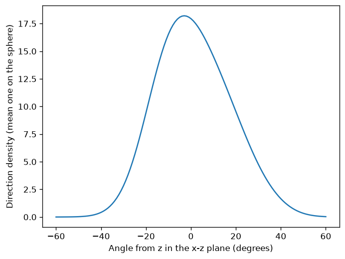
Select a kernel halfwidth for grouped direction measurements and use it in a spherical density estimate. Two measurements per group share a synthetic grain direction.

import numpy as np
import matplotlib.pyplot as plt
from mtex import vector3d, degree, calcDensity
from mtex.functions.halfwidth import degreeEnergies, selectHalfwidth

rng = np.random.default_rng(4)
grainDirections = rng.normal([0, 0, 1], [0.3, 0.3, 0.05], size=(40, 3))
measurements = np.repeat(grainDirections, 2, axis=0) + rng.normal(0, 0.01, size=(80, 3))
v = vector3d(measurements).normalize()
groups = np.repeat(np.arange(40), 2)
energies = degreeEnergies(v, groups=groups, bandwidth=64, folds=8, rng=np.random.default_rng(5))
candidates = np.linspace(5, 40, 36)*degree
halfwidth = selectHalfwidth(energies, halfwidths=candidates, noiseFloor=False)
density = calcDensity(v, halfwidth=halfwidth)
theta = np.linspace(-60, 60, 121)*degree
probe = vector3d(np.sin(theta), np.zeros_like(theta), np.cos(theta))
print('Selected halfwidth (degrees):', round(float(halfwidth/degree), 2))
plt.plot(theta/degree, density(probe))
plt.xlabel('Angle from z in the x-z plane (degrees)')
plt.ylabel('Direction density (mean one on the sphere)')
plt.show()

Group ids make the forty grain groups the independent sampling units for width selection. The noise floor is switched off here to isolate UCV and keep this demonstration short; it is enabled by default. Increase the energy bandwidth when considering narrower kernels.

Selected halfwidth (degrees): 12.0

See also

degreeEnergies, calcKernel, ucvHalfwidth, lowerBoundHalfwidth, noiseFloorHalfwidth, ucvAtEdge

MATLAB’s selectHalfwidth

@article{bachmann2010mtex,
  author  = {F. Bachmann and R. Hielscher and H. Schaeben},
  title   = {Texture Analysis with MTEX - Free and Open Source Software Toolbox},
  journal = {Solid State Phenomena},
  volume  = {160},
  pages   = {63-68},
  year    = {2010},
  doi     = {10.4028/www.scientific.net/SSP.160.63},
  url     = {https://doi.org/10.4028/www.scientific.net/SSP.160.63}
}