construct a convex crystal morphology from symmetry-related lattice planes.

Syntax

cS = crystalShape(N)

Construct from face normals in a crystal frame.

cS = crystalShape(N, habitus=1, extension=(1, 1, 2))

Modify the relative distances of the crystal forms.

cS = crystalShape.hex(cs)

Construct a hexagonal prism in the frame cs.

cS = crystalShape.quartz(simple=True)

Use a simplified shape from the mineral catalogue.

Description

Each supplied Miller normal represents a crystal form: all its symmetry equivalents are generated using the point group of its crystal frame. The shape is the bounded intersection of the half spaces dot(vertex, normal) <= 1. Before the common display scaling, a face is therefore 1/norm(normal) from the origin. Lengthening a normal moves its planes inward; shortening it can move them so far outward that other planes exclude those faces entirely. Supply enough forms to enclose a finite volume.

The optional habitus and extension parameters adjust relative plane distances using the Miller indices. For habitus p > 0, a normal with indices (h, k, l) is divided by ((abs(h)*extension[0])**p + (abs(k)*extension[1])**p + (abs(l)*extension[2])**p)**(1/p) before symmetry expansion. With habitus=0 this step is skipped and extension has no effect. This changes the morphology rather than assigning an absolute size.

The vertices are initially scaled so that their largest distance from the origin is 0.5. For a centrally symmetric crystal this gives diameter one. Read or assign diameter to set a particular size, or multiply the shape by a scale factor. Areas and volumes then have the corresponding squared and cubed length units.

An orientation places the shape in specimen coordinates: ori*cS. A list of orientations gives a list of identically connected shapes; cS+position translates their vertices. Face selection uses cS[normals], while cS[k] selects one shape from a list. Face normals used for selection are in the original crystal coordinates.

Input

`N`	Miller face normals, represented by vector3d data carrying one crystalFrame; their lengths determine the relative distances of the planes

Keywords

keyword	default	description
`habitus`	`0`	nonnegative exponent controlling the relative prominence of mixed-index forms; zero preserves the supplied Cartesian normals
`extension`	`(1, 1, 1)`	three relative scale factors associated with the h, k and l indices; used only when habitus is positive

Output

`cS`	crystalShape, initially expressed in the crystal frame of N

Properties

`N`	original face normals, one per supplied crystal form
`V`	vertices as vector3d data; a list of shapes has shape (numShapes, numVertices)
`F`	face-to-vertex connectivity, with zero-based vertex indices and -1 padding
`E`	unique edges as pairs of zero-based vertex indices
`CS`	crystalFrame in which the face normals were defined
`frame`	frame of the current vertices, changing to the specimen frame after an orientation is applied
`numFaces`	number of polygonal faces, shared by every shape in a list
`numVertices`	number of vertices per shape
`diameter`	largest distance between any two vertices; assigning it rescales the vertices
`faceArea`	numeric area of each face, with one row per shape in a list
`faceCenter`	vector3d positions given by the mean of the vertices of each face
`volume`	enclosed volume, one value per shape
`habitus`	exponent used when the shape was constructed
`extension`	three index scale factors used when the shape was constructed

Example

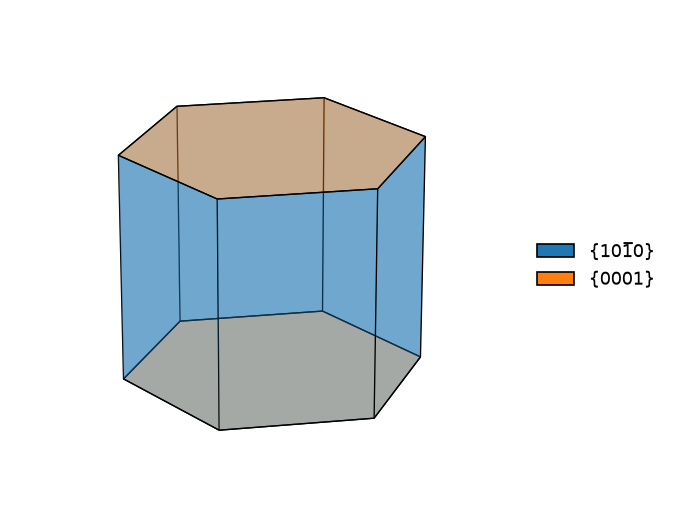
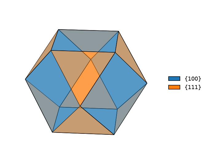
Construct a hexagonal prism without a data file, then build a cubic morphology from two families of lattice planes. Both examples use relative lengths; diameter sets the displayed size.

import matplotlib.pyplot as plt
from mtex import crystalFrame, crystalShape, Miller, cat, plot

hexagonal = crystalFrame('6/mmm', [3, 3, 4.7])
prism = crystalShape.hex(hexagonal)
prism.diameter = 2
print('Prism faces:', prism.numFaces)
plot(prism, faceAlpha=0.4, colored=True)

cubic = crystalFrame('m-3m')
normals = cat(Miller(1, 0, 0, cubic), 0.5*Miller(1, 1, 1, cubic))
truncatedCube = crystalShape(normals)
print('Truncated-cube faces:', truncatedCube.numFaces)
plot(truncatedCube, faceAlpha=0.5, colored=True)
plt.show()

The {100} planes bound the cube and the scaled {111} normals cut its corners. Changing a normal length changes its plane distance and therefore the relative prominence of that crystal form.

Prism faces: 8
Truncated-cube faces: 14

Example output for crystalShape.crystalShape

References

J. Enderlein, A package for displaying crystal morphology, Mathematica Journal 7(1), 1997

Used on

CrystalShapeSmorf, CrystalShapes

MATLAB’s crystalShape.crystalShape

source

Citing this page. This page is part of the documentation of MTEX, a free and open source MATLAB toolbox for analyzing and modeling crystallographic textures. It was written by The MTEX Developers and is published at https://mtex-toolbox.github.io/crystalShape.crystalShape_py.html. If you use MTEX, or reuse text or figures from this page, in your research, please cite

F. Bachmann, R. Hielscher, H. Schaeben: Texture Analysis with MTEX - Free and Open Source Software Toolbox, Solid State Phenomena 160 (2010), 63-68. 10.4028/www.scientific.net/SSP.160.63

BibTeX

@article{bachmann2010mtex,
  author  = {F. Bachmann and R. Hielscher and H. Schaeben},
  title   = {Texture Analysis with MTEX - Free and Open Source Software Toolbox},
  journal = {Solid State Phenomena},
  volume  = {160},
  pages   = {63-68},
  year    = {2010},
  doi     = {10.4028/www.scientific.net/SSP.160.63},
  url     = {https://doi.org/10.4028/www.scientific.net/SSP.160.63}
}

Other papers describing specific MTEX methods are listed under Publications — please cite the one that best fits your application. The MTEX source code is licensed under the GNU General Public License v2.0; the text and figures of this documentation are licensed under CC BY 4.0, which permits reuse — including by automated systems — provided The MTEX Developers and this page are credited.

crystalShape.crystalShape