Deformation Twinning

Crystal slip moves dislocations without changing the lattice orientation discontinuously. Deformation twinning instead shears part of a crystal into a second orientation related to the parent by a twin law. The transformed region is the twin domain, and its interface with the parent is a twin boundary.

A twin shear has a plane and a direction, much like a slip system. Its shear is polar: the forward sense creates or grows a twin, whereas the reverse sense can shrink an existing twin. This page uses Schmid factors to examine that loading geometry. It does not predict twin nucleation, twin volume fraction, or the full lattice reorientation.

Read Slip Systems first for plane--direction geometry and CRSS. Schmid Factor develops the stress projection used here for ordinary slip.

Define one magnesium extension-twin shear

Use a hexagonal magnesium lattice and the predefined first-order tensile twin family. The name twinT1 refers to the common \(\{10\bar{1}2\}\langle10\bar{1}1\rangle\) extension-twin mode. MTEX stores its shear direction in b, its plane normal in n, and its critical resolved shear stress (CRSS) in CRSS.

cs = crystalSymmetry('622',[3.2 3.2 5.2], ...
  'mineral','Magnesium');
sSTwin = slipSystem.twinT1(cs,1)

sSTwin = slipSystem (Magnesium)
 
  U    V    T    W  | H    K    I    L CRSS
  1   -1    0    1   -1    1    0    2    1

See the shear geometry

Draw the representative system inside a hexagonal crystal. The coloured disk is the twin plane and the arrow is the stored positive shear direction.

cS = crystalShape.hex(cs);
plot(cS,'faceAlpha',0.35,'faceColor',[0.72 0.82 0.94])
hold on
plot(cS,sSTwin,'faceColor',[0.9 0.25 0.2])
hold off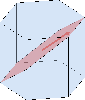

The arrow lies in the disk because the shear direction is perpendicular to the plane normal. This picture describes the local shear geometry, not the shape or thickness of a twin domain.

Resolve a tensile stress onto the shear

Apply unit tension along the crystal c-axis. The signed Schmid factor is the resolved shear stress divided by the applied stress difference. A positive value drives the stored direction; a negative value drives the reverse direction.

cAxis = Miller(0,0,0,1,cs,'UVTW');
sigmaTension = stressTensor.uniaxial(cAxis);
mTension = sSTwin.SchmidFactor(sigmaTension)

mTension =
    0.4990

Reverse the sign of the stress tensor to represent c-axis compression. Merely replacing cAxis by -cAxis would still construct the same uniaxial tensile tensor, because an axis has no positive end.

sigmaCompression = -sigmaTension;
mCompression = sSTwin.SchmidFactor(sigmaCompression)

mCompression =
   -0.4990

The two factors are 0.4990 and -0.4990. Their equal magnitude and opposite signs show the polarity directly. An ordinary slip analysis often compares absolute values because dislocations can move in either sense.

Map the loading directions

Omitting the load returns a spherical function of the tension direction. Plotting it shows where this representative receives positive and negative resolved shear.

SFTwin = sSTwin.SchmidFactor;
plot(SFTwin,'upper')
mtexColorbar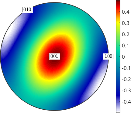

Warm and cool lobes have equal shape but opposite sign. Directions on a zero contour do not resolve shear along this stored twin direction. A large absolute value gives favourable geometry, but activation still requires the resolved shear to reach the measured CRSS.

Generate symmetry-equivalent entries

A crystal offers symmetry-related planes and directions. By default, symmetrise also retains both signs of each shear direction because the slipSystem class is shared with ordinary slip.

sSTwinAll = sSTwin.symmetrise
numberOfEntries = length(sSTwinAll)

sSTwinAll = slipSystem (Magnesium)
 size: 12 × 1
 
   U    V    T    W  | H    K    I    L CRSS
   1   -1    0    1   -1    1    0    2    1
  -1    1    0   -1   -1    1    0    2    1
   1    0   -1   -1   -1    0    1   -2    1
  -1    0    1    1   -1    0    1   -2    1
   1    0   -1    1   -1    0    1    2    1
  -1    0    1   -1   -1    0    1    2    1
   1   -1    0   -1   -1    1    0   -2    1
  -1    1    0    1   -1    1    0   -2    1
   0    1   -1    1    0   -1    1    2    1
   0   -1    1   -1    0   -1    1    2    1
   0   -1    1    1    0    1   -1    2    1
   0    1   -1   -1    0    1   -1    2    1
numberOfEntries =
    12

The twelve entries are six geometric systems with two opposite shear directions each. This is convenient for reversible slip calculations, but it is not by itself a physical list of twelve extension-twin variants. The option 'antipodal' collapses the two signs when only the geometric planes and directions are required.

sSTwinGeometry = sSTwin.symmetrise('antipodal');
numberOfGeometricSystems = length(sSTwinGeometry)

numberOfGeometricSystems =
     6

A polarity trap

Do not automatically take abs(SchmidFactor) and call its maximum the active twin variant. That operation discards the forward shear sense. Conversely, the sign chosen for an antipodal geometric representative is only a storage convention and cannot restore the missing polarity.

A physical activation model must supply the admissible signed variants, their CRSS values, and a kinetic rule for nucleation, growth, and possible detwinning. Temperature, strain rate, grain constraint, interfaces, and prior deformation can all change the observed activity. The Schmid factor is therefore a geometric screening quantity, not proof that a twin forms.

Move between crystal and specimen frames

In an experiment, the applied stress is expressed in the specimen frame. An orientation maps the crystal-frame twin shear into that frame. The two equivalent routes below either rotate the system forward or rotate the stress back into the crystal frame.

ori = orientation.byEuler(20*degree,35*degree,10*degree,cs);
sigmaSpecimen = stressTensor.uniaxial(vector3d.Z);

sSTwinSpecimen = ori * sSTwin;
mSpecimenRoute = sSTwinSpecimen.SchmidFactor(sigmaSpecimen)

sigmaCrystal = inv(ori) * sigmaSpecimen;
mCrystalRoute = sSTwin.SchmidFactor(sigmaCrystal)

mSpecimenRoute =
    0.2156
mCrystalRoute =
    0.2156

The two values agree to numerical roundoff. This equivalence is the useful check for a frame-correct EBSD calculation: rotate every candidate system by its grain orientation, or rotate the common specimen stress back into each grain's crystal frame, but do not mix the two frames.

frameRouteDifference = abs(mSpecimenRoute-mCrystalRoute)

frameRouteDifference =
   1.3878e-16

The difference is \(1.3878\times10^{-16}\), which is numerical roundoff.

From shear activity to a twin boundary

The shear system and the twin law answer different questions. A shear system tests whether a load favours a deformation mode. A twin law is the discrete orientation relationship expected between the parent and the reoriented domain. Twinning constructs that relationship and explains its symmetry-equivalent rotation angles.

Finding the same relationship across an EBSD boundary makes that boundary a candidate twin boundary. It does not prove the deformation mechanism or identify which side is the parent. Twinning Analysis combines the full misorientation with boundary morphology and explains those limitations.

% Close generated figures before the closing sections.
close all

References

Next

Continue with Twinning to turn a known twin law into an orientation relationship. For an EBSD-first workflow, use Twinning Analysis to infer and map candidate twin boundaries from their measured misorientations.

References

- J. W. Christian and S. Mahajan, Deformation Twinning, Progress in Materials Science 39 (1995), 1--157, develops the shear geometry, polarity, crystallography, and mechanics of deformation twins.
- U. F. Kocks, C. N. Tomé and H.-R. Wenk, Texture and Anisotropy, Cambridge University Press, 1998, relates resolved shear, CRSS, and deformation-system activity in textured polycrystals.