The Spherical Bingham Distribution

The Bingham distribution is a compact model for axes on the sphere. An axis has no preferred sign, so its density is antipodally symmetric: the directions \(\mathbf{v}\) and \(-\mathbf{v}\) always have the same value. This makes the model useful when measurements describe lines or planes rather than signed vectors.

The preceding Harmonic Representation page used many coefficients to describe a general shape. A Bingham distribution instead uses three perpendicular principal axes and three concentration parameters.

import numpy as np

from mtex import *

plottingConvention.default('y↑→x')

Construct one Bingham distribution

MTEX stores the concentration parameters as Z = [z1, z2, z3]. Adding the same constant to all three parameters does not change the normalized density, so the largest is conventionally set to zero. The other two are nonpositive.

The vector3d array a contains three perpendicular principal axes. A random rotation below turns the coordinate axes together while preserving their orthogonality.

Z = [-10, -4, 0]
a = rotation.rand() * vector3d.cat(xvector, yvector, zvector)
bingFun = S2FunBingham(Z, a)

plot(bingFun)
mtexColorbar()

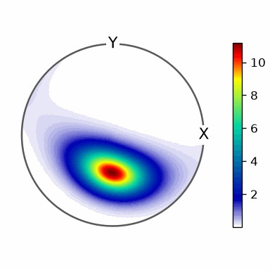
The density has equal maxima at the two ends of a[2] because its third concentration parameter is zero. The value decreases more rapidly toward a[0] than toward a[1] because -10 is more negative than -4. The contours around each maximum are therefore elongated rather than circular.

quadratureMean = mean(bingFun)
quadratureMean

1

MTEX scales a Bingham density to a mean value of one over the sphere. The port computes its normalization constant exactly, as a hypergeometric function of the matrix argument, so the mean is one. Sampling and the locations of the contours do not depend on this constant.

How the concentration parameters change the shape

The next grid uses Z = [-k1, -k2, 0] with nonnegative magnitudes \(k_1\geq k_2\). The five values 0, 4, 8, 12, and 24 show the transition from a uniform density to point maxima and girdles.

Equal values \(k_1=k_2>0\) give rotationally symmetric point maxima around the third axis. Setting \(k_2=0\) leaves a girdle: a band around the great circle perpendicular to the first axis.

kappa = [0, 4, 8, 12, 24]
mtexFig = newMtexFigure(layout=[len(kappa), len(kappa)])
for k2 in kappa:
  for k1 in kappa:
    if k1 >= k2:
      bFun = S2FunBingham([-k1, -k2, 0])
      plot(bFun, colorRange=[0, 25], axisLabels=False)
      mtexTitle(f'$\\kappa_1=${k1}  $\\kappa_2=${k2}', fontSize=12)
    if k1 < kappa[-1] or k2 < kappa[-1]:
      nextAxis()
setColorRange('equal')
mtexFig.drawNow()

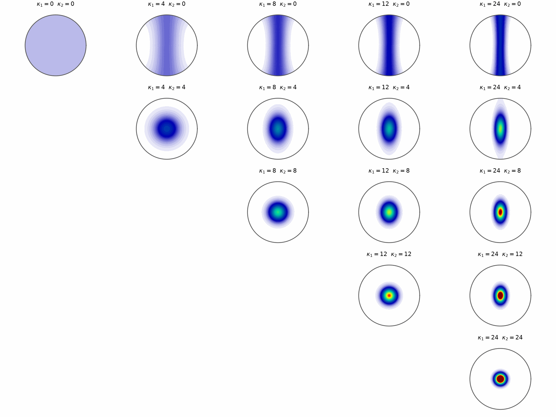
Read the grid from the uniform case at \(k_1=k_2=0\). Along the diagonal, both concentrations grow together and the two point maxima narrow. Along the \(k_2=0\) row, increasing \(k_1\) sharpens the girdle. Intermediate pairs produce elliptical contours between those two limiting shapes. Blank cells omit the redundant cases with \(k_1<k_2\).

Draw a random sample

discreteSample draws directions with probability proportional to the density.

v = bingFun.discreteSample(50)
sampleSize = v.size
sampleSize

50

plot(bingFun)
hold(True)
plot(v, markerEdgeColor='k', markerFaceColor='gray', markerFaceAlpha=0.5)
hold(False)

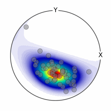
The directions cluster around both antipodal maxima and spread farther along the broad axis of the contours. The sample represents undirected axes even though each plotted point uses one signed direction.

Fit a Bingham distribution to directions

Given arbitrarily scattered directions, fit estimates the principal axes and concentrations of the best-fitting Bingham distribution. With confidenceEllipse=True it also returns the uncertainty in the fitted modal axis.

bingFunEst, ab, rot = S2FunBingham.fit(v, confidenceEllipse=True)
estimatedZ = bingFunEst.Z
estimatedZ

array([-13.4113,  -3.7401,   0.    ])

semiAxesDegrees = ab / degree
semiAxesDegrees

array([4.4586, 9.4562])

plot(bingFunEst)
hold(True)
plot(v, markerEdgeColor='k', markerFaceColor='gray', markerFaceAlpha=0.5)

# mark one representative of the fitted modal axis
annotate(bingFunEst.a[2], markerFaceColor='red', markerSize=10)

# add the default p = 0.95 confidence ellipse
ellipse(rot, ab[0], ab[1], lineWidth=3, lineColor='k')
hold(False)

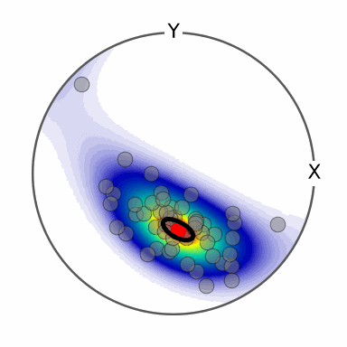
The fitted contours follow the same elongated cloud as the observations. The red marker selects bingFunEst.a[2] as one representative of the antipodal modal axis. The black ellipse is the default 95 percent confidence region for that fitted axis, not the spread of the density. The fitted Z lies close to the generating values [-10, -4, 0]; with 50 random directions it varies from one sample to the next, and so do the semi-axes of the ellipse, a few degrees each.

The method documentation calls this the confidence ellipse of the mean direction. For an antipodally symmetric distribution the vector mean vanishes, so modal axis is the more precise description. The values ab[0] and ab[1] are ellipse semi-axis lengths in radians. The rotation rot places that ellipse in the tangent plane.

The maths behind the Bingham density

Let \(A\) be the orthogonal matrix whose columns are the principal axes and let \(Z=\mathrm{diag}(z_1,z_2,z_3)\). The probability density with respect to spherical surface area is

The factor \(F(Z)\) is the exact surface-area normalization. MTEX multiplies this probability density by \(4\pi\) to use its usual mean-one density convention. Because \(\mathbf{x}^{T}\mathbf{x}=1\), adding a constant to every \(z_j\) multiplies the numerator by one constant that normalization removes. MTEX therefore uses \(z_1\leq z_2\leq z_3=0\) for the examples on this page.

The matrix \(A\) has previously been called an orthogonal covariance matrix. More precisely, it is the orthogonal matrix of principal axes. The symmetric matrix \(AZA^T\) is the concentration matrix in specimen coordinates.

References

• C. Bingham, An antipodally symmetric distribution on the sphere, The Annals of Statistics 2 (1974), 1201–1225, defines the distribution and derives estimators for its concentration and principal-axis parameters.
• T. Tanaka, Circular asymmetry of the paleomagnetic directions observed at low latitude volcanic sites, Earth, Planets and Space 51 (1999), 1279–1286, applies Bingham statistics and supplies the uncertainty construction used by fit.

Next

Continue with The Spherical Radon Transform to integrate a spherical function over the great circles perpendicular to selected directions.

Technical Details

MATLAB approximates the normalization constant by a saddle point and reports a mean of 1.0377 for these parameters; the port’s is exact. MATLAB’s fit solves for Z with the same approximation, the port’s exactly. MATLAB’s second and third outputs of fit are confidenceEllipse=True here; a[2] is MATLAB’s a(3).

@article{bachmann2010mtex,
  author  = {F. Bachmann and R. Hielscher and H. Schaeben},
  title   = {Texture Analysis with MTEX - Free and Open Source Software Toolbox},
  journal = {Solid State Phenomena},
  volume  = {160},
  pages   = {63-68},
  year    = {2010},
  doi     = {10.4028/www.scientific.net/SSP.160.63},
  url     = {https://doi.org/10.4028/www.scientific.net/SSP.160.63}
}