MTEX for Python developers

This page is for readers who know Python and want to use MTEX inside their own code: a package, a pipeline or a notebook that also uses NumPy, SciPy and matplotlib. It says where MTEX follows Python’s conventions, where it deliberately does not, and how to use it cleanly as a library.

Why the names follow MATLAB

MTEX has been a MATLAB toolbox for twenty years. Its commands (calcGrains, plotPF, symmetrise), its classes (vector3d, orientation, crystalFrame) and its options (minPixel, antipodal) are the vocabulary of its documentation, of the papers that use it and of the forum answers. The Python port keeps that vocabulary, so every page of this documentation exists in both languages and a MATLAB script translates line by line (MTEX in MATLAB and in Python). The price is a naming style that differs from PEP 8: commands and properties are in camelCase, and most classes start with a lower case letter. Libraries that mirror an established system do the same, PySide’s setWindowTitle or SimpleITK’s ReadImage.

Where a MATLAB name is a misnomer, a duplicate, a workaround for a limit of MATLAB or a typo, Python has a better one and only that: plotPF for plotPF, which draws no density when given orientations, keywords written positively as thinning=False for the flag 'nothinning', and one spelling tol= for a tolerance. The page MTEX in MATLAB and in Python lists them.

Everything below the names is ordinary Python: NumPy arrays, keyword arguments, exceptions, docstrings and matplotlib figures.

Importing

The pages of this documentation start with from mtex import *, which keeps the examples short and close to MATLAB. In code of your own, import the module or the names you use:

import numpy as np
import mtex
from mtex import calcGrains, degree, mtexdata

The package has one flat namespace: every public command, class and constant is an attribute of mtex, whichever of its layers (mtex.geometry, mtex.functions, mtex.maps, …) defines it.

mtex.orientation is mtex.geometry.orientation

True

A star import brings in min, max, sum and round too. They act on MTEX objects and fall back to Python’s built-ins on everything else, so plain values behave as before:

from mtex import max as mtexMax
mtexMax([1, 3, 2]), mtexMax(1, 5), mtexMax(x * x for x in range(4))

(3, 5, 9)

Importing MTEX takes about 0.2 s above NumPy. SciPy’s heavier modules, numba, matplotlib, h5py and PySide6 are imported only by the commands that need them.

Installation extras

The core needs NumPy, SciPy and finufft. The rest are extras of the mtex package:

A library that only computes can depend on mtex[numba] and leave the drawing out.

Containers are NumPy arrays

Every MTEX list, a list of vectors, rotations, orientations or Miller indices, holds one NumPy array of shape (..., k): k coordinates per element and any shape in front. The container’s own shape is the shape in front; one element is a container of shape ().

v = mtex.vector3d(np.random.default_rng(0).random((4, 3)))
v.shape, v.data.shape, v[0].shape

((4,), (4, 3), ())

data is the stored array: quaternions for rotations, xyz for vectors. The coordinates a reader expects have their own properties and commands:

r = mtex.rotation.byEuler(10 * degree, 20 * degree, 30 * degree)
v.xyz.shape, r.data, r.matrix()

((4, 3), array([ 0.9254,  0.171 , -0.0302,  0.3368]), array([[ 0.7713, -0.6337,  0.0594],
       [ 0.6131,  0.7146, -0.3368],
       [ 0.171 ,  0.2962,  0.9397]]))

The containers index, reshape and broadcast as NumPy arrays do, and elementwise products broadcast their shapes:

R = mtex.rotation.rand(5, rng=np.random.default_rng(1))
(R * v.reshape(4, 1)).shape

(4, 5)

NumPy sees a container as its stored coordinates: np.asarray(v) is v.data without a copy, so a container can be handed to any function that takes an array. The arithmetic stays with MTEX: an array times a container is the container’s product, and NumPy’s elementwise functions (np.sqrt, np.isnan, …) refuse a container rather than act on its coordinates.

np.asarray(v) is v.data, type(np.full(4, 2.0) * v).__name__

(True, 'vector3d')

Build a container back from an array with its constructor.

Properties and methods

A property is a stored or cheaply derived value and is written without parentheses; every is... predicate is a property too. A computation is a method with parentheses, and is also a module command:

ebsd = mtexdata('forsterite')
ori = ebsd['Forsterite'].orientations[0:3]
ori.antipodal, ori.angle(), mtex.angle(ori)

(False, array([0.8892, 0.8887, 0.8908]), array([0.8892, 0.8887, 0.8908]))

Options are keyword arguments with their MTEX names. A positional string names something: the kind of Miller indices, an Euler convention, an alignment.

mtex.Miller(1, 1, 0, ori.CS, 'uvw', antipodal=True)

vector3d (Forsterite)
  antipodal: true
  u  v  w
  1  1  0

Every public command, class and method has a docstring, so help(calcGrains), the editor’s hover and completion work. The methods MTEX attaches to classes from other modules are declared in the class bodies, so a static type checker and an editor see them without running the package.

Frames are compared by identity

A crystal or specimen frame is a handle: constructing the same frame twice returns the same object, and MTEX compares frames with is. Objects carry their frames, and the frames carry the point group.

mtex.crystalFrame('m-3m', mineral='Iron') is mtex.crystalFrame('m-3m', mineral='Iron')

True

Commands that change their input

Most commands return new objects. The exception to know is calcGrains, which writes the grain ids and the pixels it removes or absorbs into the map it is given. Pass a copy when the original must stay as it was:

grains = calcGrains(ebsd.copy(), angle=10 * degree, minPixel=5)
len(grains)

885

Session state

MTEX keeps one session per Python process: the preferences of setMTEXpref and the register of frames. A preference changes the behaviour of every caller in the process. The preferences a user saves with save=True go to mtex_settings.json and are read at import; a library or a test that must see the defaults whatever the user saved sets the environment variable MTEX_SETTINGS to an empty string before importing MTEX. mtex.reset() returns the session to its defaults; a preference that is not set prints as None.

mtex.setMTEXpref('kernels', 'numpy')
mtex.getMTEXpref('kernels')

'numpy'

mtex.reset()
print(mtex.getMTEXpref('kernels'))

None

The preference threads sets the threads of numba, finufft and scipy.fft; by default it is the number of physical cores. The compiled kernels can be called from several Python threads at once.

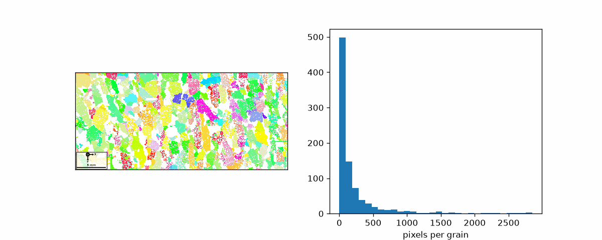
Plots are matplotlib

The plotting commands draw with matplotlib and return its artists. parent= draws into an axes of your own, so MTEX plots sit beside any other matplotlib content:

import matplotlib.pyplot as plt

fig, (left, right) = plt.subplots(1, 2, figsize=(10, 4))
mtex.plot(ebsd['Forsterite'], ebsd['Forsterite'].orientations, parent=left)
right.hist(grains.grainSize, bins=30)
right.set_xlabel('pixels per grain')

Stability

The names of commands, classes and options are fixed from 1.0 on; internals, everything whose name starts with an underscore and the modules not re-exported by mtex, can change between releases.

@article{bachmann2010mtex,
  author  = {F. Bachmann and R. Hielscher and H. Schaeben},
  title   = {Texture Analysis with MTEX - Free and Open Source Software Toolbox},
  journal = {Solid State Phenomena},
  volume  = {160},
  pages   = {63-68},
  year    = {2010},
  doi     = {10.4028/www.scientific.net/SSP.160.63},
  url     = {https://doi.org/10.4028/www.scientific.net/SSP.160.63}
}