Successive Refinement of Pole Figure Reconstructions

ODF Estimation reconstructs an orientation distribution function (ODF) on one orientation grid with one kernel width. A kernel is the smooth component placed at each grid orientation. Its width sets the smallest scale that the reconstruction can represent.

This page refines two different parts of that workflow. First, calcODFIterative keeps the measurements fixed while it successively narrows the kernel. Second, a simulation keeps the reconstruction method fixed while it adds measurements where the current ODF predicts high pole density.

Successive kernel refinement is not the same as asking calcODF for more solver iterations. It changes the representation scale and uses each coarser solution to initialise the next one. Neither kind of refinement removes the non-uniqueness of pole figure inversion; see The Ghost Effect.

import numpy as np
from mtex import *

Adapting the kernel

The seven measured Dubna pole figures provide a reference case. The ordinary reconstruction solves directly at its target resolution.

plottingConvention.default('y↑→x')
pf = mtexdata('dubna')
odf_naive = calcODF(pf)

calcError(pf, odf_naive)

array([0.3912, 0.3243, 0.237 , 0.2872, 0.2895, 0.3601, 0.3229])

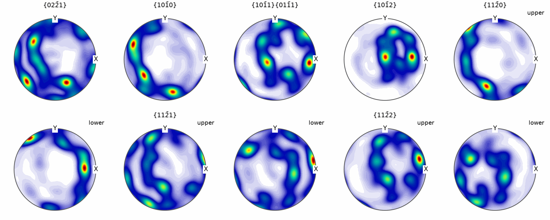
The seven values are the fit errors for the seven measured pole figures. Their recalculated pole figures are the visual baseline for the iterative result below.

plotPF(odf_naive, pf.allH)

The iterative reconstruction starts from a uniform ODF. It solves first with a wide kernel, transfers those weights to a finer grid, narrows the kernel, and solves again. The coarse stages suppress fine-scale variation and provide informed starting weights for the finer stages.

This scale progression acts as a regularisation strategy for irregularly sampled data. It does not replace ghost correction. The thinning=False flag retains low-weight grid nodes so that this comparison isolates the effect of the changing scale.

odf_iter = calcODFIterative(pf, thinning=False, verbose=True)

calcError(pf, odf_iter)

   0 | 0.91  0.93  0.74  0.79  0.93  0.85  0.77
   1 | 0.89  0.89  0.74  0.71  0.89  0.84  0.76
   2 | 0.88  0.88  0.74  0.68  0.88  0.83  0.75
   3 | 0.87  0.86  0.73  0.66  0.87  0.82  0.75
   4 | 0.87  0.86  0.73  0.65  0.86  0.82  0.74
   5 | 0.87  0.85  0.73  0.64  0.85  0.81  0.74
   6 | 0.86  0.85  0.73  0.64  0.85  0.81  0.74
   1 :      46 | 0.56  0.50  0.43  0.48  0.48  0.53  0.49
   0 | 0.88  0.87  0.74  0.67  0.87  0.82  0.75
   1 | 0.86  0.84  0.70  0.63  0.84  0.80  0.72
   2 | 0.85  0.81  0.68  0.59  0.81  0.79  0.69
   3 | 0.84  0.79  0.66  0.57  0.79  0.77  0.67
   4 | 0.83  0.77  0.65  0.56  0.77  0.76  0.66
   5 | 0.82  0.77  0.64  0.55  0.76  0.76  0.65
   6 | 0.81  0.76  0.64  0.55  0.76  0.75  0.65
⋮
   4 :    4635 | 0.29  0.19  0.23  0.18  0.17  0.27  0.28
   0 | 0.60  0.57  0.39  0.23  0.46  0.49  0.39
   1 | 0.56  0.57  0.40  0.17  0.40  0.46  0.36
   2 | 0.57  0.55  0.37  0.18  0.41  0.46  0.36
   3 | 0.55  0.55  0.38  0.16  0.39  0.45  0.35
   4 | 0.57  0.55  0.36  0.18  0.40  0.45  0.36
   5 | 0.55  0.55  0.37  0.16  0.39  0.44  0.35
   6 | 0.56  0.54  0.36  0.17  0.40  0.45  0.35
   5 :   20040 | 0.29  0.19  0.22  0.18  0.17  0.27  0.28
array([0.2924, 0.1908, 0.2215, 0.1801, 0.1667, 0.2699, 0.2779])

One fit error is reported per pole figure. All seven are smaller than those from the ordinary reconstruction, in places by nearly a factor of two.

plotPF(odf_iter, pf.allH)

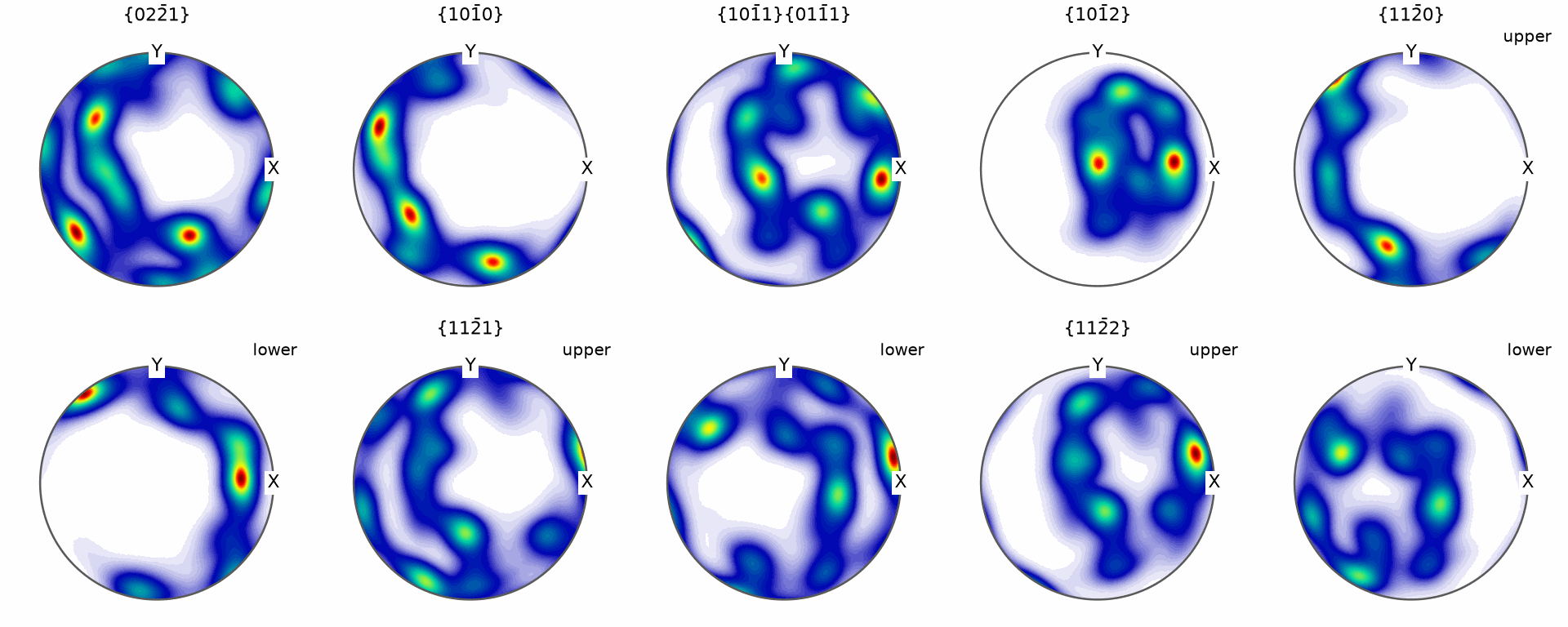
The peak positions in the two galleries are similar. The error values show that their intensities are not, so a visual match alone is not enough to compare reconstructions. Their L1 difference measures how much ODF volume is distributed differently.

calcError(odf_iter, odf_naive, 'l1')

0.1484

Fifteen percent of the volume sits in different places in the two reconstructions. Recalculating pole figures from their signed difference shows where that volume moved. The printed values give the minimum, mean, and maximum difference over all seven pole figures.

pf_difference = calcPoleFigure(odf_naive - odf_iter, pf)
plot(pf_difference)
differenceIntensity = pf_difference.intensities
print(f'pole figure difference min / mean / max : {np.min(differenceIntensity):.2f} / {np.mean(differenceIntensity):.2f} / '
      f'{np.max(differenceIntensity):.2f}')

pole figure difference min / mean / max : -0.90 / 0.00 / 0.55

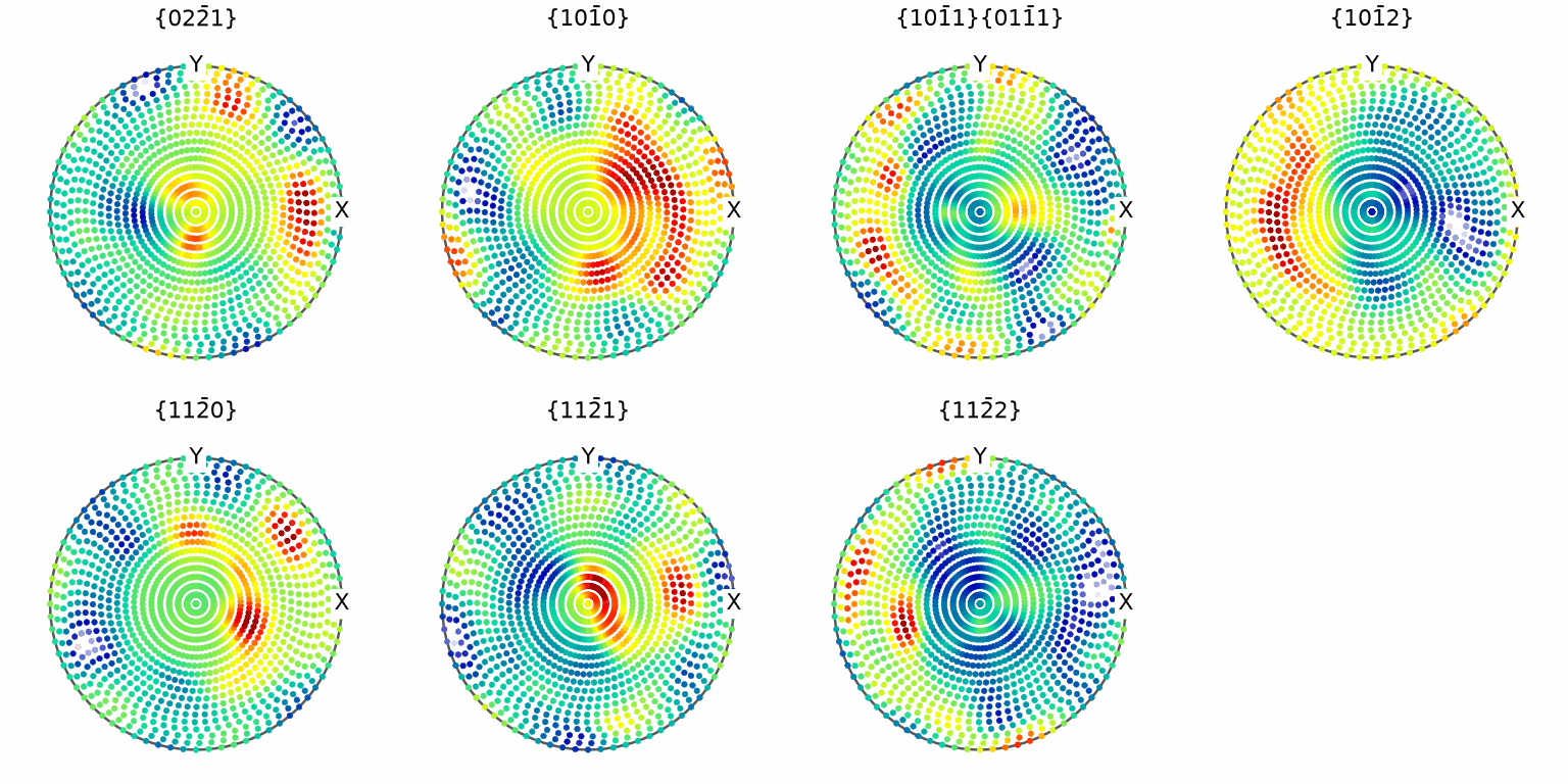
The range from -0.92 to 0.58 is centred at 0.00. Broad, smooth differences extend across the sphere instead of concentrating at the texture maxima. Compare the centre of each pole figure with its rim.

This is the appearance of a differently distributed uniform portion. It is the part of an ODF that pole figures constrain least, which is why a smaller fit error does not prove that the reconstructed ODF is closer to the unknown true ODF.

Adapting the measurement

The rest of the page uses a simulation so that the true ODF is known. Simulating Pole Figure Data develops this validation strategy. Here the model has two sharp components, and pole figures can be evaluated at whichever specimen directions are selected.

cs = crystalFrame('cubic')
plottingConvention.default('y↑→x')
ss = specimenFrame()

q = rotation.byEuler(10 * degree, 10 * degree, 10 * degree, 'ABG')
q2 = rotation.byEuler(10 * degree, 30 * degree, 10 * degree, 'ABG')

odf_true = .6 * unimodalODF(q, cs, ss, halfwidth=5 * degree) + .4 * unimodalODF(q2, cs, ss, halfwidth=4 * degree)

Three lattice planes will be measured.

h = Miller([[1, 1, 1], [1, 0, 0], [1, 1, 0]], cs)

plotPF(odf_true, h)

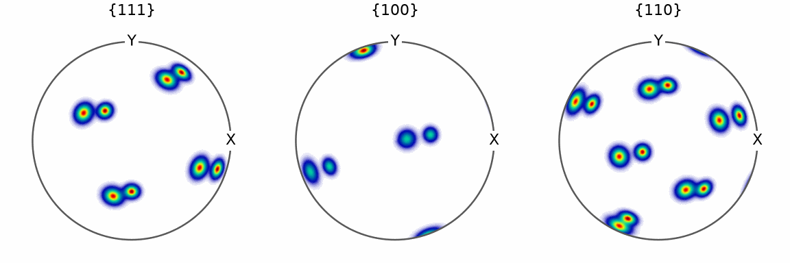
The compact maxima reflect the 4 and 5 degree component halfwidths. They are the features that a coarse measurement must first locate and then sample more densely.

The initial measurement grid

The first scan uses a nearly equispaced 15 degree grid out to a specimen tilt of 80 degrees.

r = equispacedS2Grid(resolution=15 * degree, maxTheta=80 * degree)

plot(r, markerSize=12, upper=True)

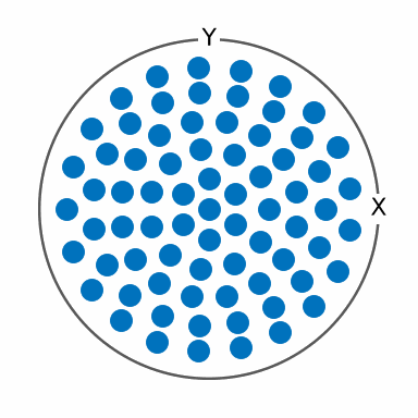
The points cover the accessible cap uniformly. The gaps between them are deliberately much wider than the sharp model components.

The refinement loop

Each round measures the current directions and merges them with all earlier measurements. An ordinary reconstruction then predicts the pole density at the directions inserted by refine. Only the quarter with the highest predicted intensity is measured in the next round. Five rounds are used here.

This highest-intensity rule is deliberately naive. It exploits the current estimate but does not account for uncertainty, counting noise, acquisition cost, or the possibility that the current estimate missed a component. It demonstrates adaptive sampling, not a general experimental design prescription.

r = [equispacedS2Grid(resolution=15 * degree, maxTheta=80 * degree)] * h.size
pf_measured = None
nsteps = 5

for k in range(nsteps):

  # simulate the new measurements
  pf_simulated = calcPoleFigure(odf_true, h, r)

  # merge new and previous measurements
  pf_measured = union(pf_simulated, pf_measured)
  plot(pf_measured)

  meanResolution = np.mean([x.resolution for x in pf_measured.allR])
  print(f'- mean sampling resolution : {meanResolution / degree:f}')

  if k < nsteps - 1:
    # reconstruct from all measurements collected so far
    odf_recalc = calcODF(pf_measured, zeroRange=True)
    print(f'  error true -- estimated odf   : {calcError(odf_true, odf_recalc):f}')

    # select high-intensity directions from the refined grids
    for l in range(h.size):
      r_old = pf_measured[l].r
      _, r_new = refine(r_old)
      pf_predicted = calcPoleFigure(odf_recalc, h[l], r_new)
      threshold = np.nanquantile(pf_predicted.intensities, 0.75)
      r[l] = pf_predicted.r[pf_predicted.intensities > threshold]

- mean sampling resolution : 15.270088
  error true -- estimated odf   : 0.816625
- mean sampling resolution : 13.540635
  error true -- estimated odf   : 1.004866
- mean sampling resolution : 9.755493
  error true -- estimated odf   : 0.657554
- mean sampling resolution : 7.548409
  error true -- estimated odf   : 0.384405
- mean sampling resolution : 4.166612

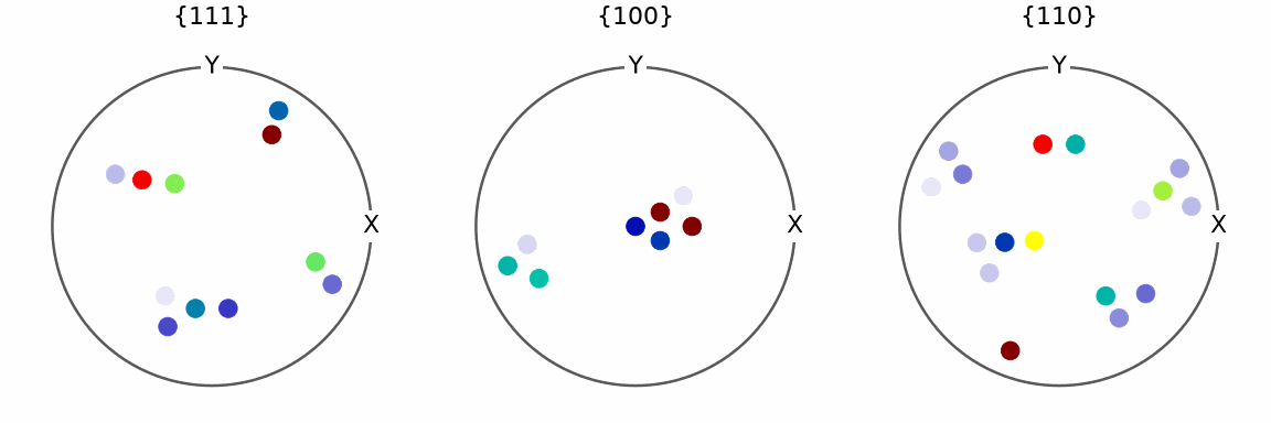
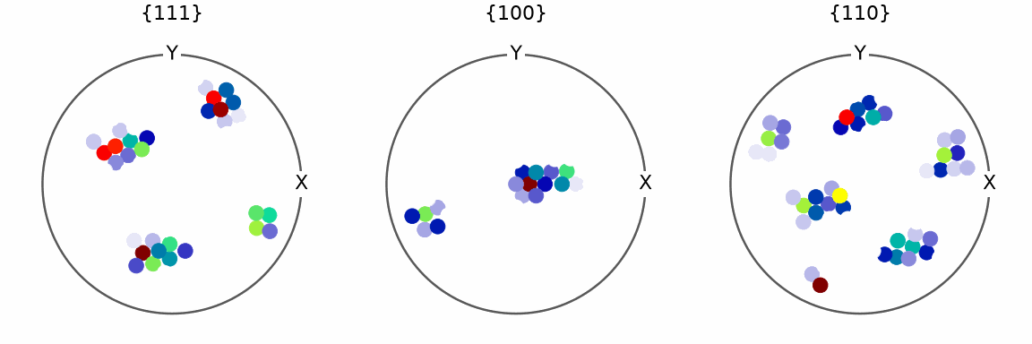
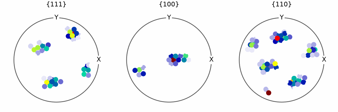
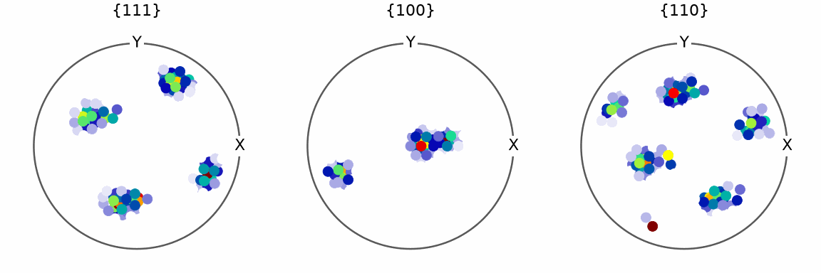
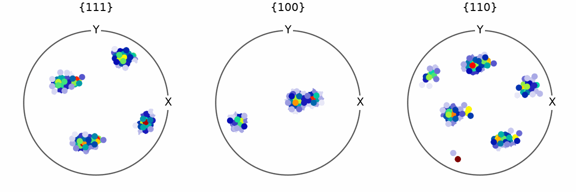
Every round prints the mean resolution of the three accumulated direction sets. This single value summarises an irregular sampling pattern; it does not mean that neighbouring points are that far apart everywhere.

The mean resolution falls from 15.3 to 4.3 degrees. The four interim ODF errors are 0.82, 1.01, 0.66, and 0.47. They do not fall monotonically: the second round concentrates the new directions on the predicted maxima before the reconstruction has located them accurately. A real experiment could not compute these errors because its true ODF is unknown.

That non-monotonicity is the point of the demonstration. The measurement is now dense where the texture is strong and coarse everywhere else. An ordinary fine-grid reconstruction then puts ODF components at orientations that the sparse regions do not constrain.

What was measured

The object summary gives the number of accumulated directions for each pole figure. The sampling pattern is no longer a regular grid.

pf_measured

PoleFigure (m3̅m → y↑→x)
  h = {111}, r = 327 points
  h = {100}, r = 327 points
  h = {110}, r = 327 points

plot(pf_measured)

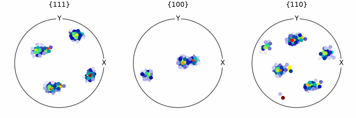
Dense clusters surround the predicted poles of the two components. The original coarse coverage remains between them. This uneven coverage is exactly the case for which successive kernel refinement is useful. Within each cluster, the colours rise towards a predicted pole-density maximum.

Reconstructing from the irregular measurement

First use an ordinary reconstruction at the 2.5 degree resolution that the dense regions can support.

odf_recalc = calcODF(pf_measured, zeroRange=True, resolution=2.5 * degree)
print(f'  error true -- estimated odf   : {calcError(odf_true, odf_recalc):f}')

  error true -- estimated odf   : 0.239274

The iterative reconstruction reaches the same target scale through a sequence of wider kernels. Sparse regions inherit the broad distribution established at coarse scale instead of being determined only at the finest scale.

odf_recalc_iterative = calcODFIterative(pf_measured, halfwidth=2.5 * degree)
print(f'  error true -- iter. est. odf  : {calcError(odf_true, odf_recalc_iterative):f}')

  error true -- iter. est. odf  : 0.115130

The errors are 0.22 for the direct reconstruction and 0.12 for the iterative one. The iterative error is about half the direct error from the same measurements. The L1 distance below shows how much the two estimated ODFs distribute differently.

calcError(odf_recalc, odf_recalc_iterative, 'l1')

0.1708

About a sixth of the volume is placed differently. On an unevenly sampled measurement, the choice between a direct fine-scale solve and successive refinement is therefore part of the model, not an implementation detail.

Further reading

• R. Hielscher and H. Schaeben, A Novel Pole Figure Inversion Method: Specification of the MTEX Algorithm, Journal of Applied Crystallography 41 (2008), 1024-1037. This paper derives the component method used by calcODF for sharp textures and irregular specimen directions.
• F. Bachmann, Texturbestimmung aus Beugungsbildern, in Optimierung der Goniometrie zur Texturbestimmung aus Röntgenbeugungsbildern, Springer Spektrum, 2016, pp. 79-106. This chapter describes the reconstruction strategy behind calcODFIterative.
• ASTM International, ASTM E81-96(2024): Standard Test Method for Preparing Quantitative Pole Figures. This standard covers X-ray acquisition procedures. It does not prescribe an inversion method or the adaptive sampling rule demonstrated here.

Next

Simulating Pole Figure Data adds counting noise and asks how many pole figures a reconstruction needs. Then return to The Ghost Effect for the information that no refinement of measurement density can recover.

Technical Details

union takes None for the empty data set MATLAB starts from, and pf_measured[l] is MATLAB’s pf_measured{l}. calcODFIterative prints its ladder of grids and fit errors with silent=False.

Two things make the refinement loop take a different path from MATLAB’s. A pole figure derives the resolution of its specimen directions from the points, as the square root of the median area of their Voronoi cells, where MATLAB remembers the spacing the grid was built with, so the first round reports 15.3 degrees rather than 14.5. And refine keeps a cap a cap: it returns the centroids of the Delaunay triangles of the points, none below the lowest one, where MATLAB closes the hull with the south pole and keeps the centroids of the skirt triangles as well. The accumulated measurement therefore ends at 327 directions per pole figure rather than 367, all of them inside the measured cap.

@article{bachmann2010mtex,
  author  = {F. Bachmann and R. Hielscher and H. Schaeben},
  title   = {Texture Analysis with MTEX - Free and Open Source Software Toolbox},
  journal = {Solid State Phenomena},
  volume  = {160},
  pages   = {63-68},
  year    = {2010},
  doi     = {10.4028/www.scientific.net/SSP.160.63},
  url     = {https://doi.org/10.4028/www.scientific.net/SSP.160.63}
}