Crystal Directions
Crystal directions are directions relative to a crystal reference frame and are usually defined in terms of Miller indices. This sections explains how to calculate with crystal directions in MTEX.
| On this page ... |
| Definition |
| Trigonal and Hexagonal Convention |
| Symmetrically Equivalent Crystal Directions |
| Angles |
| Conversions |
| Calculations |
Definition
Since crystal directions are always subject to a certain crystal reference frame, the starting point for any crystal direction is the definition of a variable of type crystalSymmetry
cs = crystalSymmetry('triclinic',[5.29,9.18,9.42],[90.4,98.9,90.1]*degree,...
  'X||a*','Z||c','mineral','Talc');
The variable cs containes the geometry of the crystal reference frame and, in particular, the alignment of the crystallographic a,b, and, c axis.
a = cs.aAxis
b = cs.bAxis
c = cs.cAxis
a = Miller
 size: 1 x 1
 mineral: Talc (-1, X||a*, Z||c)
  u 1
  v 0
  w 0

b = Miller
 size: 1 x 1
 mineral: Talc (-1, X||a*, Z||c)
  u 0
  v 1
  w 0

c = Miller
 size: 1 x 1
 mineral: Talc (-1, X||a*, Z||c)
  u 0
  v 0
  w 1
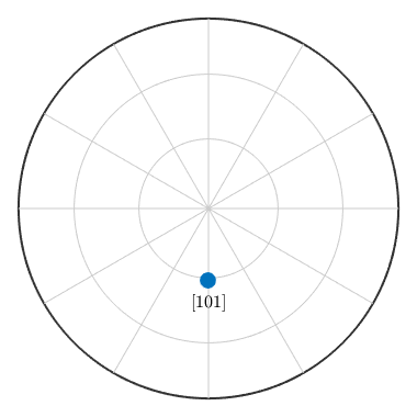
A crystal direction m = u * a + v * b + w * c is a vector with coordinates u, v, w with respect to these crystallographic axes. In MTEX a crystal direction is represented by a variable of type Miller which is defined by
m = Miller(1,0,1,cs,'uvw')m = Miller size: 1 x 1 mineral: Talc (-1, X||a*, Z||c) u 1 v 0 w 1
for values u = 1, v = 0, and, w = 1. To plot a crystal direction as a spherical projections do
plot(m,'upper','labeled','grid')
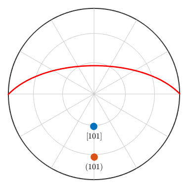
Alternatively, a crystal direction may also be defined in the reciprocal space, i.e. with respect to the dual axes a*, b*, c*. The corresponding coordinates are usually denoted by h, k, l. Note that for non Euclidean crystal frames uvw and hkl notations usually lead to different directions.
m = Miller(1,0,1,cs,'hkl')
hold on
plot(m,'upper','labeled')
% the corresponding lattice plane
plot(m,'plane','linecolor','r','linewidth',2)
hold off
m = Miller
 size: 1 x 1
 mineral: Talc (-1, X||a*, Z||c)
  h 1
  k 0
  l 1
Trigonal and Hexagonal Convention
In the case of trigonal and hexagonal crystal symmetry, the convention of using four Miller indices h, k, i, l, and U, V, T, W is supported as well.
cs = loadCIF('quartz')
m = Miller(2,1,-3,1,cs,'UVTW')
cs = crystalSymmetry

  mineral        : Quartz
  symmetry       : 321
  a, b, c        : 4.9, 4.9, 5.4
  reference frame: X||a*, Y||b, Z||c*


m = Miller
 size: 1 x 1
 mineral: Quartz (321, X||a*, Y||b, Z||c*)
  U  2
  V  1
  T -3
  W  1
Symmetrically Equivalent Crystal Directions
A simple way to compute all symmetrically equivalent directions to a given crystal direction is provided by the command symmetrise
symmetrise(m)
ans = Miller
 size: 6 x 1
 mineral: Quartz (321, X||a*, Y||b, Z||c*)
  U  2  2 -3 -3  1  1
  V  1 -3  2  1 -3  2
  T -3  1  1  2  2 -3
  W  1 -1  1 -1  1 -1
As always the keyword antipodal adds antipodal symmetry to this computation
symmetrise(m,'antipodal')ans = Miller size: 12 x 1 mineral: Quartz (321, X||a*, Y||b, Z||c*) U 2 2 -3 -3 1 1 -2 -2 3 3 -1 -1 V 1 -3 2 1 -3 2 -1 3 -2 -1 3 -2 T -3 1 1 2 2 -3 3 -1 -1 -2 -2 3 W 1 -1 1 -1 1 -1 -1 1 -1 1 -1 1
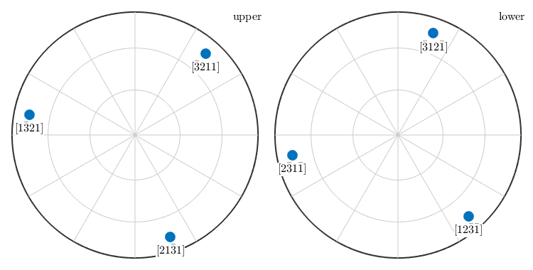
Using the options symmetrised and labeled all symmetrically equivalent crystal directions are plotted together with their Miller indices.
plot(m,'symmetrised','labeled','grid','backgroundcolor','w')
The command eq or == can be used to check whether two crystal directions are symmetrically equivalent. Compare
Miller(1,1,-2,0,cs) == Miller(-1,-1,2,0,cs)
ans =
  logical
   0
and
eq(Miller(1,1,-2,0,cs),Miller(-1,-1,2,0,cs),'antipodal')ans = logical 1
Angles
The angle between two crystal directions m1 and m2 is defined as the smallest angle between m1 and all symmetrically equivalent directions to m2. This angle is in radians and it is calculated by the function angle
angle(Miller(1,1,-2,0,cs),Miller(-1,-1,2,0,cs)) / degree
ans =
   60.0000
As always the keyword antipodal adds antipodal symmetry to this computation
angle(Miller(1,1,-2,0,cs),Miller(-1,-1,2,0,cs),'antipodal') / degreeans =
0
Conversions
Converting a crystal direction which is represented by its coordinates with respect to the crystal coordinate system a, b, c into a representation with respect to the associated Euclidean coordinate system is done by the command vectord3d.
vector3d(m)
ans = vector3d
 size: 1 x 1
        x       y       z
  7.09563   2.458  1.8018
Conversion into spherical coordinates requires the function polar
[theta,rho] = polar(m)
theta =
    1.3353
rho =
    0.3335
Calculations
Essentially all the operations defined for general directions, i.e. for variables of type vector3d are also available for Miller indices. In addition Miller indices interact with crystal orientations. Consider the crystal orientation
o = orientation.byEuler(10*degree,20*degree,30*degree,cs)
o = orientation
  size: 1 x 1
  crystal symmetry : Quartz (321, X||a*, Y||b, Z||c*)
  specimen symmetry: 1

  Bunge Euler angles in degree
  phi1  Phi phi2 Inv.
    10   20   30    0
Then one can apply it to a crystal direction to find its coordinates with respect to the specimen coordinate system
o * m
ans = vector3d
 size: 1 x 1
        x       y       z
  4.02206  5.4999 3.63462
By applying a crystal symmetry one obtains the coordinates with respect to the specimen coordinate system of all crystallographically equivalent specimen directions.
p = o * symmetrise(m);
plot(p,'grid')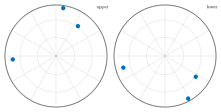
| DocHelp 0.1 beta |