Antipodal Symmetry

Directions vs. Axes

In MTEX it is possible to consider three dimensional vectors either as directions or as axes. The key option to distinguish between both interpretations is antipodal.

Consider a pair of vectors

v1 = vector3d(1,1,2);
v2 = vector3d(1,1,-2);

and plots them in a spherical projection

plot([v1,v2],'label',{'v_1','v_2'})

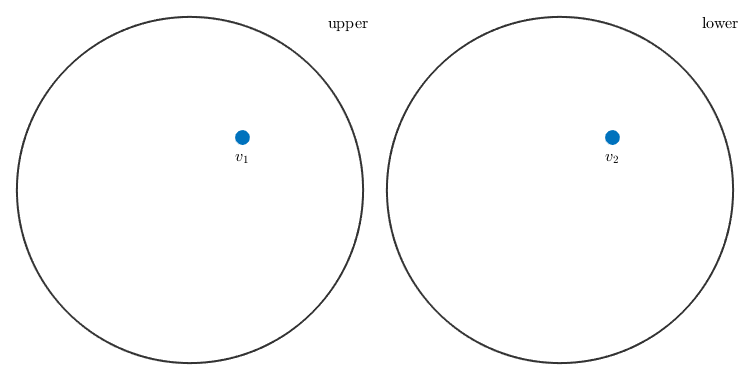
These vectors will appear either on the upper or on the lower hemisphere. In order to treat these vectors as axes, i.e. in order to assume antipodal symmetry - one has to use the keyword antipodal.

plot([v1,v2],'label',{'v_1','v_2'},'antipodal')

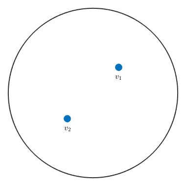
Now the direction v_2 is identified with the direction -v_2 which plots at the upper hemisphere.

Back to Top

The Angle between Directions and Axes

Another example, where antipodal symmetry matters is the angle between two vectors. In the absence of antipodal geometry we have

angle(v1,v2) / degree

ans =
  109.4712

whereas, if antipodal symmetry is assumed we obtain

angle(v1,v2,'antipodal') / degree

ans =
   70.5288

Back to Top

Antipodal Symmetry in Experimental Pole Figures

Due to Friedel's law experimental pole figures always provide antipodal symmetry. One consequence of this fact is that MTEX plots pole figure data always on the upper hemisphere. Moreover if you annotate a certain direction to pole figure data, it is always interpreted as an axis, i.e. projected to the upper hemisphere if necessary

mtexdata dubna

% plot the first pole figure
plot(pf({1}))

% annotate a axis on the souther hemisphere
annotate(vector3d(1,0,-1),'labeled','backgroundColor','w')

 loading data ...
 saving data to /home/hielscher/mtex/master/data/dubna.mat

Back to Top

Antipodal Symmetry in Recalculated Pole Figures

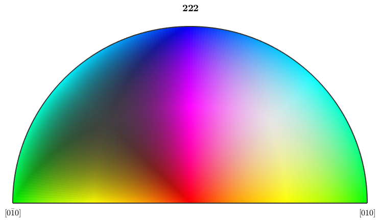
However, in the case of pole figures calculated from an ODF antipodal symmetry is in general not present.

% some prefered orientation
o = orientation.byEuler(20*degree,30*degree,0,'ZYZ',CS);

% define an unimodal ODF
odf = unimodalODF(o);

% plot pole figures
plotPDF(odf,[Miller(1,2,2,CS),-Miller(1,2,2,CS)])

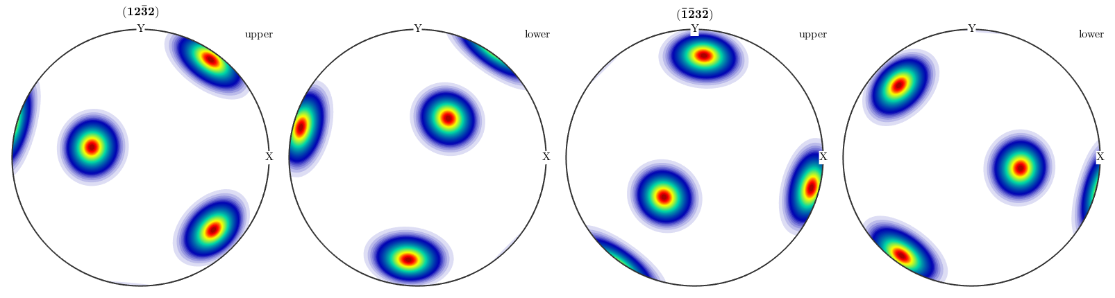
Hence, if one wants to compare calculated pole figures with experimental ones, one has to add antipodal symmetry.

plotPDF(odf,Miller(1,2,2,CS),'antipodal')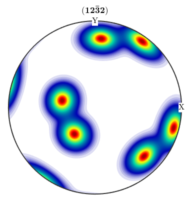

Back to Top

Antipodal Symmetry in Inverse Pole Figures

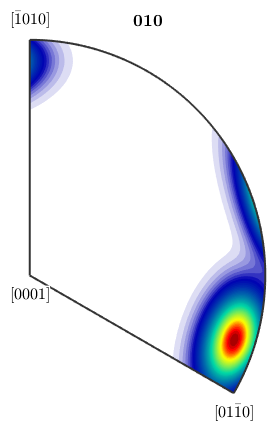
The same reasoning as above holds true for inverse pole figures. If we look at complete, inverse pole figures they do not posses antipodal symmetry in general

plotIPDF(odf,[yvector,-yvector],'complete')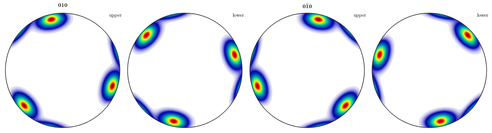

However, if we add the keyword antipodal, antipodal symmetry is enforced.

plotIPDF(odf,yvector,'antipodal','complete')

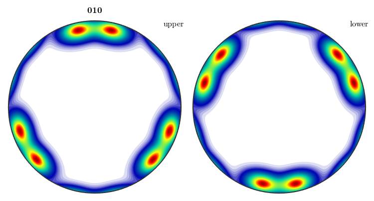
Notice how MTEX, automatically reduces the fundamental region of inverse pole figures in the case that antipodal symmetry is present.

plotIPDF(odf,yvector)

plotIPDF(odf,yvector,'antipodal')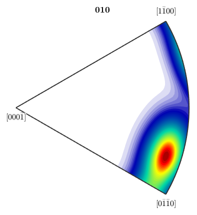

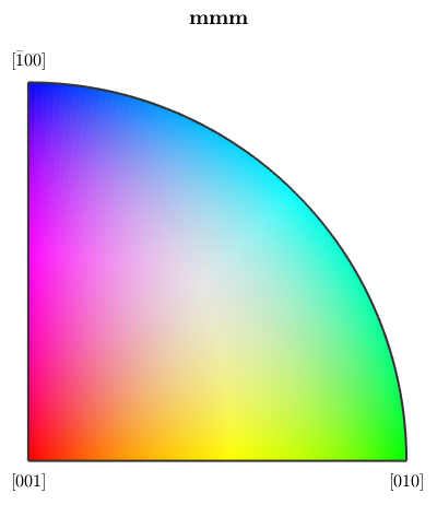
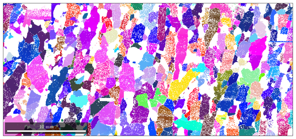
Back to Top

EBSD Colocoding

Antipodal symmetry effects also the colocoding of ebsd plots. Let's first import some data.

mtexdata forsterite

Now we plot these data with a colorcoding according to the inverse (100) pole figure. If we use the Laue group for inverse pole figure color coding we add antipodal symmetry to the inverse pole figure

ipfKey = ipfColorKey(ebsd('fo').CS.Laue);

% plot the color key
plot(ipfKey)

Here the colorized data

plot(ebsd('fo'),ipfKey.orientation2color(ebsd('fo').orientations))

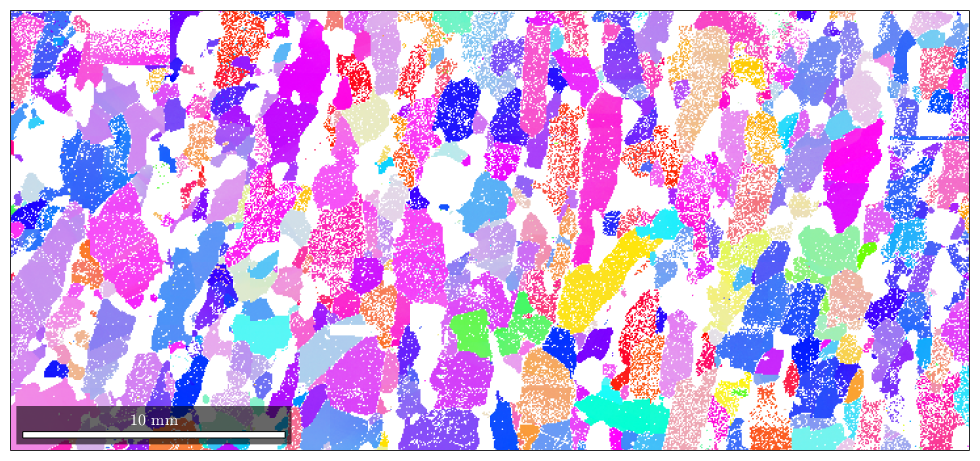
If we use the point group of proper rotations this antipodal symmetry is not present and a larger region of the inverse pole figure is colorized

ipfKey = ipfColorKey(ebsd('fo').CS.properGroup);

% the colorcode
plot(ipfKey)

Here the colorized data

plot(ebsd('fo'),ipfKey.orientation2color(ebsd('fo').orientations))

Back to Top

DocHelp 0.1 beta