
This page has no MATLAB counterpart: the key it describes exists only in the Python port. It is an option of the default key, not a replacement, and maps drawn without it look exactly as in MTEX.
The default MTEX key, described in IPF Maps, places white at the centre of the fundamental sector and the primary colours at its corners. It does not change its colour at the same rate everywhere. Measured in OKLab, a colour space in which equal distances look like equal colour differences, the colour of the cubic key changes about three times as fast per degree in some parts of the sector as in others: fast around yellow and cyan, slow near the white centre and along the red corner. Two grains a few degrees apart can therefore look alike in one part of the map and clearly different in another.
perceptual=True builds the key in OKLab instead, so that its colour changes at a nearly
steady rate over the whole sector.
import numpy as np
from mtex import *
ebsd = mtexdata('twins')
mg = ebsd['indexed']
The two keys side by side
The magnesium map below is textured close to the basal pole \([0001]\), which is exactly the red corner of the key. First the default key.
key = ipfHSVKey(mg)

plot(mg, key.orientation2color(mg.orientations))
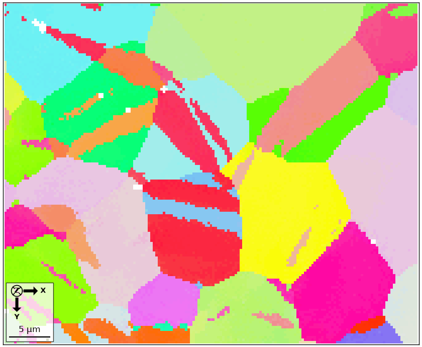
plot(key)
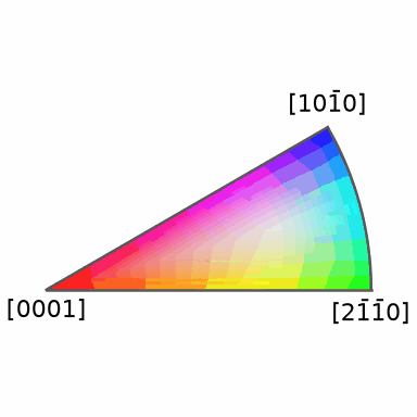
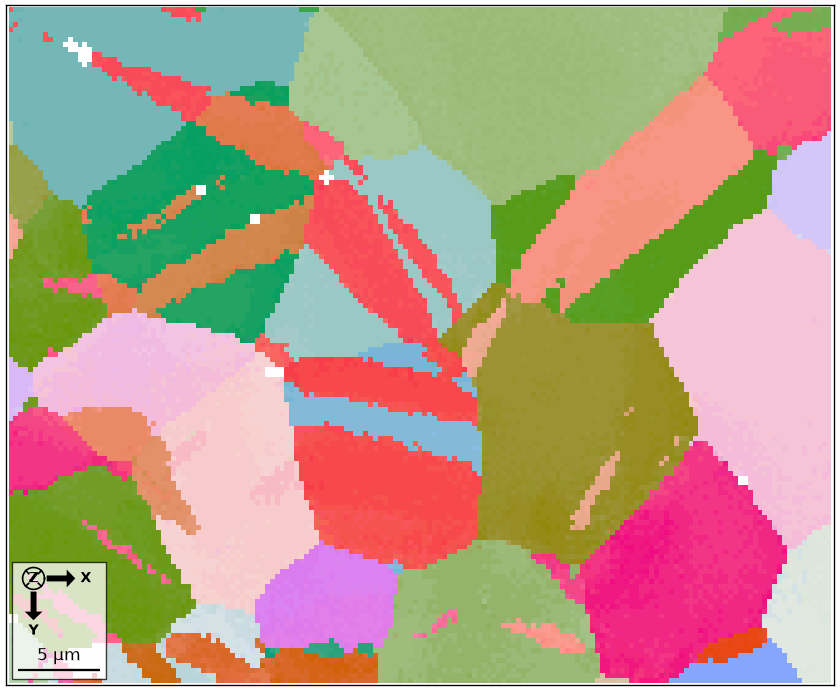
Now the perceptual key. Its sector is the same, its white centre is the same and its corners keep red, green and blue; only the colours in between are placed differently.
key = ipfHSVKey(mg, perceptual=True)

plot(mg, key.orientation2color(mg.orientations))
plot(key)
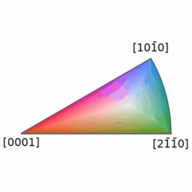
The red grain in the middle, the pink grains beside it and the salmon twin lamellae stay apart, the pale grains near the white centre differ more than before, and no single grain grabs the eye merely because it sits where the default key is most saturated. The price is visible too: yellow cannot be both saturated and as dark as the rest of the key’s boundary, so the large yellow grain becomes olive.
Letting the lightness follow the hue
In sRGB every hue has a lightness at which it is most saturated: yellow is brightest at
an OKLab lightness of 0.96, cyan at 0.90, green at 0.86, magenta at 0.70, red at 0.62
and blue at 0.50. A key that holds one lightness for all hues along its boundary gives
up the bright yellows and cyans; a key that follows these values keeps them, but its
lightness now jumps between neighbouring hues, and the colour changes fastest exactly
there. hueLightness, from 0 to 1, chooses between the two.
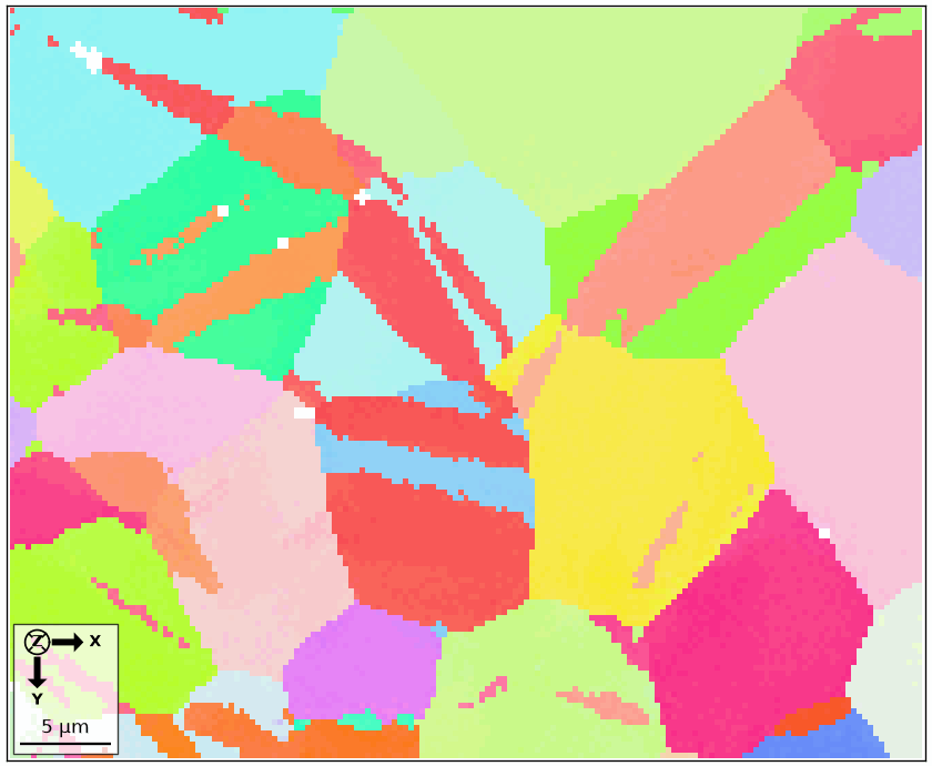
key = ipfHSVKey(mg, perceptual=True, hueLightness=1)

plot(mg, key.orientation2color(mg.orientations))
plot(key)
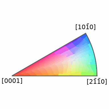
With hueLightness=1 the yellow grain is yellow again and the map comes close to the
default key, slightly softer. This is not a coincidence: MTEX’s key, built on the HSL
colour sphere, effectively already places every hue at its most saturated lightness,
and much of its unevenness is that choice. Intermediate values give intermediate keys.
How even the keys are can be read off one number, the ratio of the fastest to the slowest colour change in the sector (the 90th over the 10th percentile of the OKLab colour difference per degree, at random directions of the sector; 1 would be perfectly even):
| point group | MTEX | perceptual=True |
hueLightness=0.5 |
hueLightness=1 |
|---|---|---|---|---|
| m-3m | 3.06 | 1.80 | 2.44 | 2.60 |
| 6/mmm | 3.12 | 2.19 | 2.33 | 2.65 |
| -3m | 3.91 | 2.18 | 2.18 | 3.17 |
| 4mm | 3.07 | 1.81 | 2.47 | 2.96 |
The mean colour change per degree, the contrast the key gives, is about the same for all of them: 0.023 for the perceptual cubic key and 0.022 for MTEX’s.
Other point groups
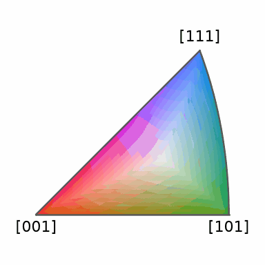
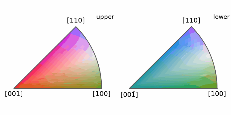
The option applies wherever the default key does, for every point group and for the groups without inversion, whose sector the key splits into a white and a dark half.
plot(ipfHSVKey(crystalFrame('m-3m'), perceptual=True))
plot(ipfHSVKey(crystalFrame('4mm'), perceptual=True))
The maths behind the perceptual key
The sector geometry is the one of the default key: every direction gets a radius \(r\), 1 at the white centre and 0 on the boundary, and an azimuth \(\rho\) about the centre, equalised so that the corners of a triangle land at \(0\), \(2\pi/3\) and \(4\pi/3\). Only the step from \((r, \rho)\) to a colour differs. In OKLab coordinates \((L, a, b)\) with the chroma \(C\) and the hue \(h\), \(a = C\cos h\), \(b = C\sin h\),
\[L = L_w + (L_b(h) - L_w)\,(1 - r), \qquad C = C_b(h)\,(1 - r), \qquad h = \eta(\rho),\]a cone with its apex at the white centre, \(L_w = 0.95\). For the groups without inversion the cone continues past the boundary to a dark apex at \(L = 0.30\).
- \(\eta\) passes through the OKLab hues of red, yellow, green, cyan, blue and magenta at every sixth of the turn. OKLab gives red to yellow 81 degrees of hue and yellow to green only 33, so a hue turning evenly with \(\rho\) would give red two thirds of that side of the sector.
- \(L_b(h)\) is 0.62 for every hue at
hueLightness=0and moves to the lightness of the hue’s largest saturation ashueLightnessgoes to 1. - \(C_b(h)\) is, at each hue, the largest chroma for which the whole cone stays inside the sRGB gamut, so the key is never clipped.
Along the radius the lightness and the chroma both change linearly, and along the arc the hue does, so for a fixed hue the colour changes at a constant rate. What remains uneven comes from \(C_b(h)\) and \(L_b(h)\) varying with the hue, and from the sector geometry itself.
Technical Details
The spread numbers are measured on the colour keys directly, with 8000 random
directions of the fundamental sector and two perpendicular steps of 0.15 degrees; the
test test_the_perceptual_key in tests/test_directionkeys.py checks their order.
The tables \(L_b(h)\) and \(C_b(h)\) are computed once per value of hueLightness, on first
use. OKLab is the colour space of B. Ottosson, A perceptual color space for image
processing, 2020.
Next
IPF Maps develops the default key this page varies. Sharp Color Keys spends the whole key on a small orientation range.
Citing this page.
This page is part of the documentation of
MTEX, a free and open
source MATLAB toolbox for analyzing and modeling crystallographic textures.
It was written by The MTEX Developers and is published at
https://mtex-toolbox.github.io/EBSDPerceptualKey_py.html.
If you use MTEX, or reuse text or figures from this page, in your research,
please cite
F. Bachmann, R. Hielscher, H. Schaeben: Texture Analysis with MTEX - Free and Open Source Software Toolbox, Solid State Phenomena 160 (2010), 63-68. 10.4028/www.scientific.net/SSP.160.63
BibTeX
@article{bachmann2010mtex,
  author  = {F. Bachmann and R. Hielscher and H. Schaeben},
  title   = {Texture Analysis with MTEX - Free and Open Source Software Toolbox},
  journal = {Solid State Phenomena},
  volume  = {160},
  pages   = {63-68},
  year    = {2010},
  doi     = {10.4028/www.scientific.net/SSP.160.63},
  url     = {https://doi.org/10.4028/www.scientific.net/SSP.160.63}
}
Other papers describing specific MTEX methods are listed under Publications — please cite the one that best fits your application. The MTEX source code is licensed under the GNU General Public License v2.0; the text and figures of this documentation are licensed under CC BY 4.0, which permits reuse — including by automated systems — provided The MTEX Developers and this page are credited.