
Authors: Vivian Tong; Stefan Olovsjö, Seco Tools AB, R&D Materials and Technology, 737 82 Fagersta, Sweden. Contact: vivian.tong@extern.tu-freiberg.de
An EBSD map and an SEM image of the same area never quite line up. The beam drifts during the scan, the camera moves between acquisitions, the specimen is tilted. Overlay the two and features are out by tens of pixels, which is enough to ruin any measurement that needs both.
TrueEBSD corrects that, so every pixel of the map and every pixel of the images refer to the same point on the sample. The method is described in Tong et al., arXiv 2605.00703.
This page uses trueEbsd, which is part of MTEX - nothing has to be installed alongside it, and it asks for no toolbox that MTEX does not already require. Expect minutes rather than seconds: this is the full field of view.
The short version runs the same five maps and the same four distortions on a cut-down copy in well under a minute. Start there if you are new to it; this page is the full field of view, and adds the two things that dataset is too small to show - a map stored the other way round from its images, and a matching window set badly enough to need a retry.
The data
An EBSD map of a WC-Co composite taken at 20 kV, and four SEM images of the same area, all in ebsd.opt.trueEbsdImgs:
-
fsdB3— colour image from the three FSD detectors below the EBSD camera, camera retracted 20 mm from the mapping position;
-
fsdT3— the same beam scan asfsdB3, from the FSD detectors above the camera;
-
fsdT1— top FSD detectors, camera at the mapping position;
-
fsdT10— asfsdT1, but with the beam at 10 kV.
pixSzImg is their pixel size in microns, the same for all four. The map itself is represented by its band contrast, ebsd.bc.
The convention set here only decides which way up the figures come out. It has no effect on the correction.
plottingConvention.default('y↓→x')

mtexdata trueEbsdWCCo

display(ebsd.opt.trueEbsdImgs)
ans = plottingConvention (y↓→x)
ebsd = EBSDsquare (y↓→x, col←row↓)
Phase Orientations Mineral Color Symmetry Crystal reference frame
0 6657 (0.85%) notIndexed none
1 714592 (91%) W C LightSkyBlue -6m2 X||a*, Y||b, Z||c
2 62791 (8%) Co-fcc DarkSeaGreen m-3m
3 2392 (0.3%) Co-hcp Goldenrod 6/mmm X||a*, Y||b, Z||c
Properties: bc, bs, bands, MAD, quality, oldId
Scan unit : um
X × Y × Z : [0 → 41] × [0 → 30] × [0 → 0]
Normal vector: (0,0,1)
Square grid :768 × 1024
struct with fields:
fsdB3: [1536×2048×3 double]
fsdT3: [1536×2048 double]
fsdT1: [1536×2048 double]
fsdT10: [1536×2048 double]
pixSzImg: 0.0199Build the sequence
TrueEBSD does not jump straight from the EBSD map to the reference image. It steps through the images one pair at a time, correcting one kind of distortion at each step. That is the point of having four images rather than one: each pair differs by something simple enough to model, where the map and the final image differ by everything at once.
So the order matters. It runs from the most distorted to the ground truth. The distortions themselves go in a second list further down, one per hop, so the images say only what they are.
The reference image is the one you trust: here fsdT10, taken at the mapping position. Everything is brought onto it.
'name' is what each image will be called once it is attached to the map at the end, so you read the result as ebsd.fsdT1.
img = ebsd.opt.trueEbsdImgs;

imgList = [mapImage(ebsd.bc, ebsd,             'name','bcImg'), ...
           mapImage(img.fsdB3,  'dxy',img.pixSzImg, 'name','fsdB3'), ...
           mapImage(img.fsdT3,  'dxy',img.pixSzImg, 'name','fsdT3'), ...
           mapImage(img.fsdT1,  'dxy',img.pixSzImg, 'name','fsdT1'), ...
           mapImage(img.fsdT10, 'dxy',img.pixSzImg, 'name','fsdT10')]
imgList = mapImage (y↓→x)
image pixel frame layout name EBSD
1 768 × 1024 0.04 um y↓→x col←row↓ bcImg W C, Co-fcc, Co-hcp
2 1536 × 2048 × 3 0.02 um iY↓→iX row↓→col fsdB3 -
3 1536 × 2048 0.02 um iY↓→iX row↓→col fsdT3 -
4 1536 × 2048 0.02 um iY↓→iX row↓→col fsdT1 -
5 1536 × 2048 0.02 um iY↓→iX row↓→col fsdT10 -A light box filter first — cross-correlation dislikes noise — and one common range, since the levels off different detectors mean nothing to each other. Both are methods of mapImage and both take the whole list at once. Neither needs the Image Processing Toolbox.
imgList(2:end) = rescale(imboxfilt(imgList(2:end),3));The distortions are objects, one per hop, not names on the images. Five maps means four hops, and the reference has no entry of its own — where nothing separates a pair that is spatialTransformId.
A multi-stage hop is + and not *: + reads left to right in the order the stages are applied and keeps both, where an unfitted prototype has zero coefficients, reports itself as the identity, and * would absorb it.
T = [spatialTransformShift + spatialTransformDrift, ...
     spatialTransformId, ...
     spatialTransformShift, ...
     spatialTransformTilt]
T = spatialTransform
size: 1 × 4
model stage parameters
1 shift-drift shift scale 1 × 1, rotate 0°, shear 0°, move (0, 0)
drift (no knots)
2 identity · ·
3 shift · scale 1 × 1, rotate 0°, shear 0°, move (0, 0)
4 tilt projective perspective (0, 0)
poly11 |c| = 0
poly22 |c| = 0Plot the sequence to check the images really do cover the same area. Note how different the contrasts look — that is why matching is done on edges rather than on grey values.
plot(imgList)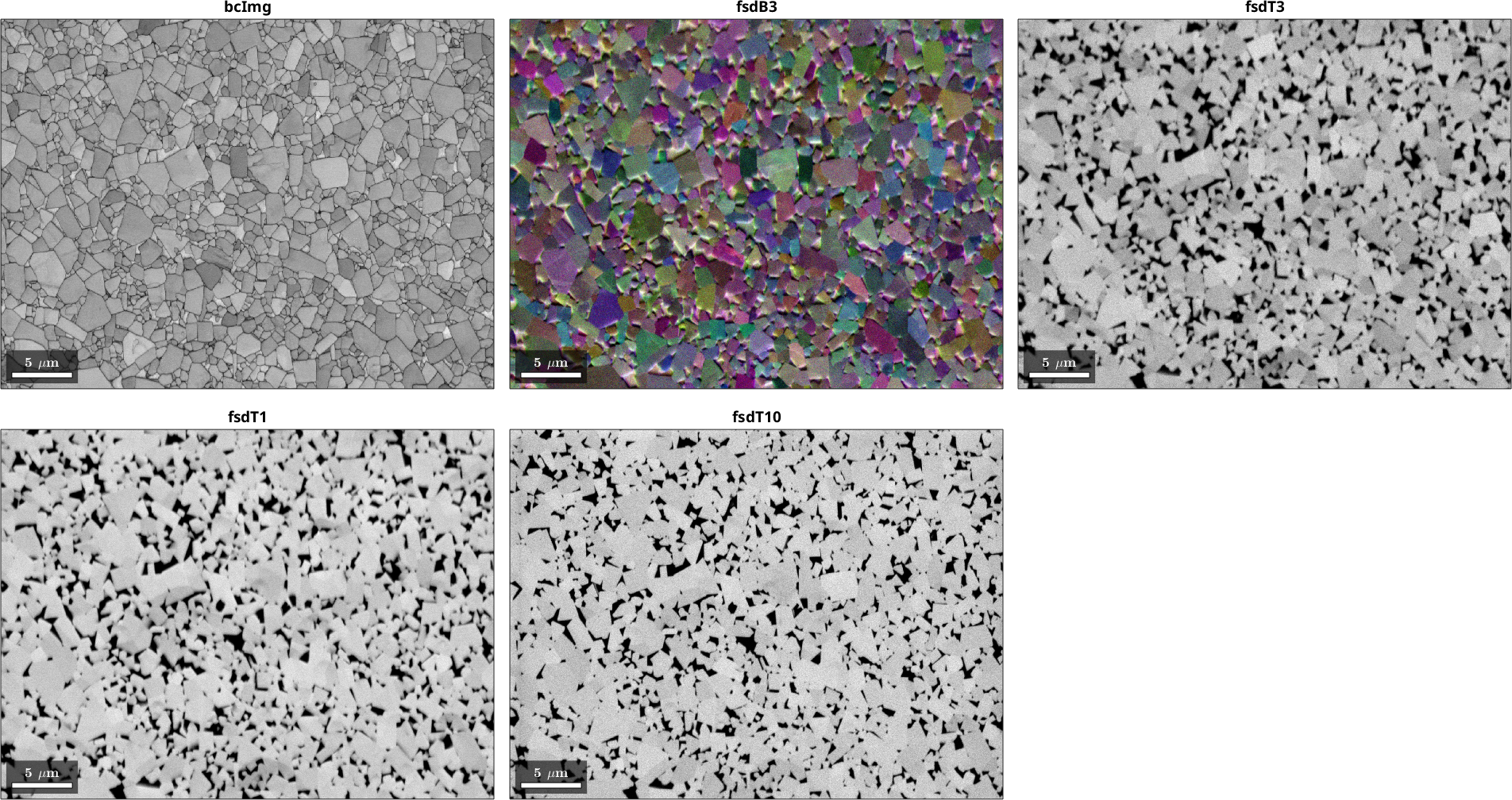
Say how the map and the images are related
Comparing two pictures pixel by pixel only means something if you know which way round each one is stored. TrueEBSD asks rather than guesses, because guessing wrong does not fail loudly — it returns a finished-looking result that is quietly nonsense.
Usually there is nothing to do: a map and images collected in one session are stored the same way and TrueEBSD confirms it. This file is the exception. Its EBSD map was written with the columns in the opposite order from the images, so pixel (1,1) of the map and pixel (1,1) of an image are at opposite ends of the sample.
You will not see this in the plot above. Every plot draws each entry the way that entry says it should be drawn, so on screen they already agree — the difference is in how the numbers are stored, and that is what matters when they are compared. transformReferenceFrame puts them all in one frame, working the relation out from what the map and the images each already say about themselves.
Where that is not enough — an image from a separate session, at an unknown rotation — you state the relation instead. See the frames page.
imgList = imgList.transformReferenceFrame(imgList(1).frame)imgList = mapImage (y↓→x)
image pixel frame layout name EBSD
1 768 × 1024 0.04 um y↓→x row↓→col bcImg W C, Co-fcc, Co-hcp
2 1536 × 2048 × 3 0.02 um y↓→x row↓→col fsdB3 -
3 1536 × 2048 0.02 um y↓→x row↓→col fsdT3 -
4 1536 × 2048 0.02 um y↓→x row↓→col fsdT1 -
5 1536 × 2048 0.02 um y↓→x row↓→col fsdT10 -Now the job can be built. It holds the whole workflow, and each step below adds to it. It also re-checks that the sequence is in one frame, and stops with trueEbsd:frameMismatch if not.
job = trueEbsd(imgList,T)job = trueEbsd (as imported)
name image distortion shift, px residual, px
1 bcImg 768 × 1024 shift-drift - -
2 fsdB3 1536 × 2048 × 3 identity - -
3 fsdT3 1536 × 2048 shift - -
4 fsdT1 1536 × 2048 tilt - -
5 fsdT10 1536 × 2048 - -Put everything on one pixel grid
The map and the images cover the same area at different pixel sizes. pixelSizeMatch resamples them all onto the finest one, so pixel (i,j) means roughly the same place in each.
Images are interpolated linearly. EBSD data is not: orientations and phase labels have no meaningful average, so the nearest measured point is used.
Nothing has been corrected yet — this is only bookkeeping.
job.pixelSizeMatchusing default pixel size of 0.019875 um, minimum from imgList
ans = trueEbsd (pixel size matched)
name image distortion shift, px residual, px
1 bcImg 1536 × 2048 shift-drift - -
2 fsdB3 1536 × 2048 × 3 identity - -
3 fsdT3 1536 × 2048 shift - -
4 fsdT1 1536 × 2048 tilt - -
5 fsdT10 1536 × 2048 - -
common grid: 1536 × 2048 at 0.02 µmThe resampled sequence is in job.resizedList.
job.resizedListans = mapImage (y↓→x)
image pixel frame layout name EBSD
1 1536 × 2048 0.02 um y↓→x row↓→col bcImg W C, Co-fcc, Co-hcp
2 1536 × 2048 × 3 0.02 um y↓→x row↓→col fsdB3 -
3 1536 × 2048 0.02 um y↓→x row↓→col fsdT3 -
4 1536 × 2048 0.02 um y↓→x row↓→col fsdT1 -
5 1536 × 2048 0.02 um y↓→x row↓→col fsdT10 -[Optional] Adjust the matching windows
Distortions are measured by cutting both images of a pair into small boxes and cross-correlating each box with its partner. That gives a local shift at each box, and those shifts are fitted to the distortion model.
Almost none of it has to be specified. roiSize — the box width — is measured from the images the first time calcDistortion needs it, from the rule of thumb that a box has to be at least four times the shift it is asked to measure and wide enough to hold several features. What was chosen is printed, so it can be overridden.
Everything here is a length, in the map's own scanUnit, so it means the same before and after pixelSizeMatch and may be set at any point. numROI is how many boxes fit across; the number down follows from the aspect ratio.
Here the second stage of the first hop is set deliberately far too small, to show what happens when the box width is wrong.
px = job.resizedList(1).dx;

% deliberately far too small on the second stage of hop 1, to show the
% retry - everything else is measured
job.setOptions('numROI',40);
job.setOptions(1,'roiSize',[64 32]*px);
job.setOptions(3,'roiSize',128*px);
job.setOptions(3:5,'registerOn','raw');
Measure the distortion
These are the pictures that will actually be matched: edge transforms where registerOn is 'edge', grey values where it is 'raw'. A band contrast map and a backscatter image have nothing in common as grey values, but their grain boundaries fall in the same places — which is why edges are the default.
plot(job.resizedList,'edge')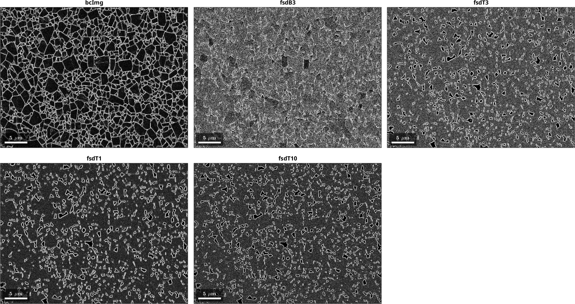
'fitErr' re-measures the shifts after each correction and reports what is left over. That residual is how you tell whether it worked: around a pixel or less is good.
The shift and residual columns each read as a length followed by the signed x and y behind it, in pixels of the common grid: how far the step moved the map, and which way. A hop that is one coherent movement — a stage that drifted, a camera that was retracted — has a direction, and the pair says what it was. Where the pair falls to nearly zero against a large length, the boxes disagree among themselves and the correlation found no common direction, which is what a step that has not worked looks like.
Because the first box size was set too small, the EBSD map step is exactly that, and leaves a residual above two pixels. TrueEBSD notices, doubles the box size and tries again, repeating until the residual comes down or the box outgrows the image. Watch the printed table.
Steps whose transform is spatialTransformId are skipped — nothing separates that pair, so their shift is taken as zero whatever the residual says.
job.calcDistortion('fitErr')◆ measured settings, override with setOptions
▸ edgeWidth per map 6 7 7 7 7 px
▸ roiSize per hop · 128 · 128 px ← shifts · 2.4 · 14.3 px, features · 13 · 13 px
◆ distortion across 5 maps, 4 hops
distortion stage ROI shift, px residual, px
──────────── ───────────── ──────── ────────────────── ──────────────────
● bcImg
│ shift-drift shift 64 px 12.13 (+2.68,+1.52)
│ drift 32 px 6.40 (+0.44,+0.74)
│ ↳ residual 5.71 (+0.52,+0.56)
│ ↻ residual over 2 px, retrying with a 128 px ROI
│ shift-drift shift 128 px 14.41 (+5.21,+1.76)
│ drift 64 px 6.40 (+0.38,-0.39)
│ ↳ residual 4.41 (+0.12,-0.22)
│ ↻ residual over 2 px, retrying with a 256 px ROI
│ shift-drift shift 256 px 14.04 (+5.46,+2.66)
│ drift 128 px 5.54 (+0.07,-0.79)
│ ↳ residual 2.39 (-0.03,+0.10)
│ ↻ residual over 2 px, retrying with a 512 px ROI
│ shift-drift shift 512 px 12.13 (+5.49,+4.79)
│ drift 256 px 5.09 (-0.01,-2.04)
│ ↳ residual 1.30 (+0.08,-0.11)
▼
● fsdB3
│ identity · · 0.00 (+0.00,+0.00)
│ ↳ difference 3.70 (+0.20,-1.74)
▼
● fsdT3
│ shift shift 128 px 12.63 (-10.51,-6.63)
│ ↳ residual 0.97 (-0.51,-0.45)
▼
● fsdT1
│ tilt projective 128 px 14.16 (+10.97,-8.12)
│ poly11 128 px 0.86 (+0.30,-0.43)
│ poly22 128 px 0.80 (+0.26,-0.07)
│ ↳ residual 0.79 (+0.26,-0.01)
▼
● fsdT10
ans = trueEbsd (shifts calculated)
name image distortion shift, px residual, px
1 bcImg 1536 × 2048 shift-drift 7.06 (+0.33,-4.86) 1.30 (+0.08,-0.11)
2 fsdB3 1536 × 2048 × 3 identity 0.00 (+0.00,+0.00) 3.70 (+0.20,-1.74)
3 fsdT3 1536 × 2048 shift 12.57 (-10.60,-6.74) 0.97 (-0.51,-0.45)
4 fsdT1 1536 × 2048 tilt 0.40 (+0.26,-0.09) 0.79 (+0.26,-0.01)
5 fsdT10 1536 × 2048 - -
common grid: 1536 × 2048 at 0.02 µmCorrect it
Each map is now moved by the shifts of every step between it and the reference. The reference itself does not move.
Resampling is nearest-neighbour throughout, so no orientation and no phase label is ever invented by averaging two real measurements.
job.undistort

plot(job.undistortedList)
ans = trueEbsd (undistorted)
name image distortion shift, px residual, px
1 bcImg 1536 × 2048 shift-drift 7.06 (+0.33,-4.86) 1.30 (+0.08,-0.11)
2 fsdB3 1536 × 2048 × 3 identity 0.00 (+0.00,+0.00) 3.70 (+0.20,-1.74)
3 fsdT3 1536 × 2048 shift 12.57 (-10.60,-6.74) 0.97 (-0.51,-0.45)
4 fsdT1 1536 × 2048 tilt 0.40 (+0.26,-0.09) 0.79 (+0.26,-0.01)
5 fsdT10 1536 × 2048 - -
common grid: 1536 × 2048 at 0.02 µm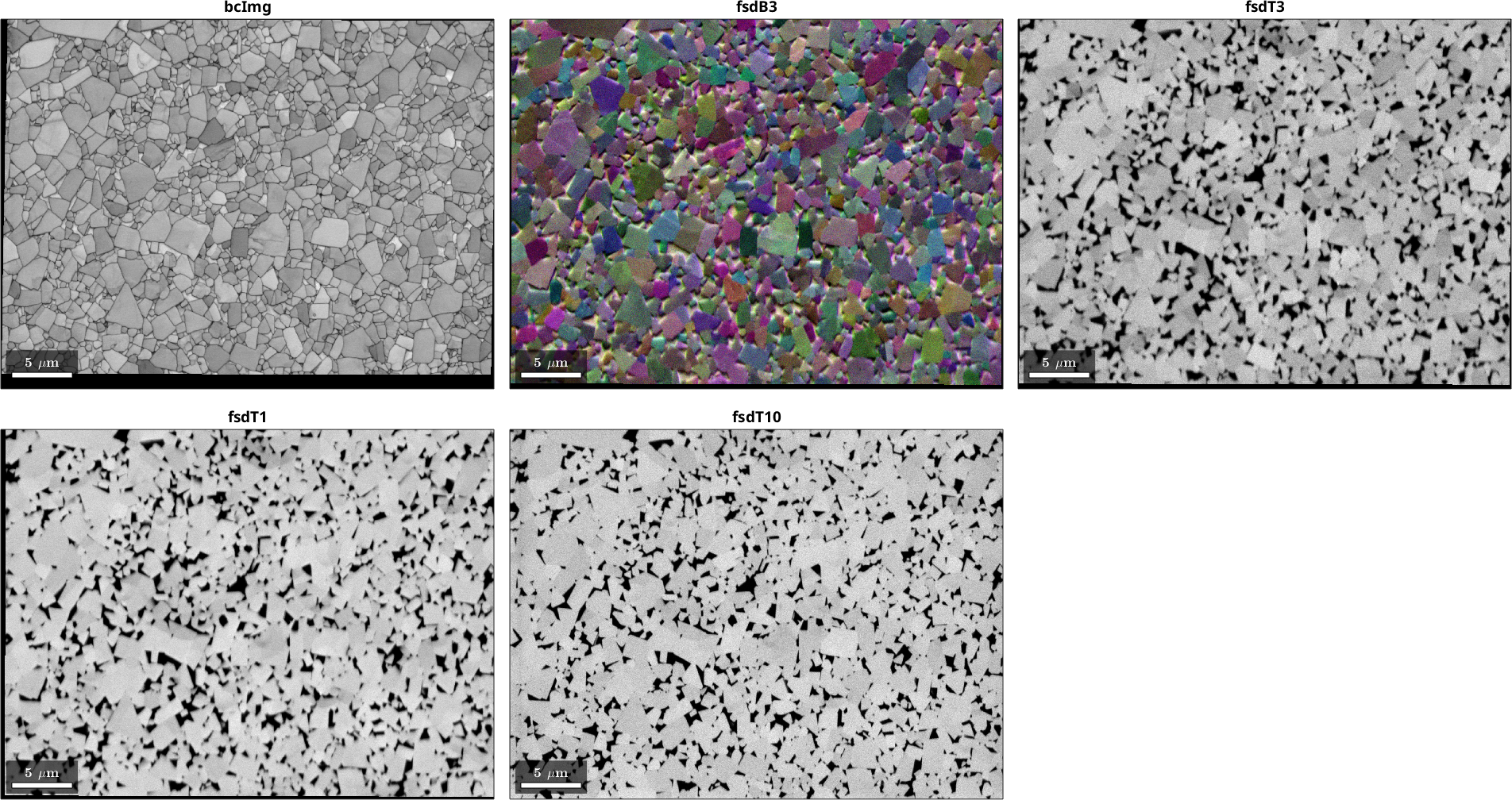
Use the result
Every image is now attached to the EBSD map as a per-pixel property, under the 'name' given earlier. So ebsd.fsdT1 is just another map property, and plot(ebsd,ebsd.fsdT1) works like any other plot — no conversion, and it stays with the map through cropping, gridding and indexing.
Plotting them back onto the map is also the quickest check that nothing came out the wrong way round.
fsdB3 is a colour image and keeps all three channels. Plotting onto a map needs one value per pixel, so it is averaged to grey here.
ebsdOut = job.undistortedList(1).ebsd;

figure
nextAxis
plot(ebsdOut('W C'), ebsdOut('W C').orientations, 'coordinates','on')
title('Undistorted MTEX EBSD map (WC IPF out of screen)','Color','k')

for n = 1:numel(job.undistortedList)

  im = ebsdOut.(job.undistortedList(n).name);
  if size(im,3) > 1, im = mean(im,3); end

  nextAxis
  plot(ebsdOut, im, 'coordinates','on')
  mtexColorMap gray
  title(['Undistorted ' job.undistortedList(n).name],'Color','k')
end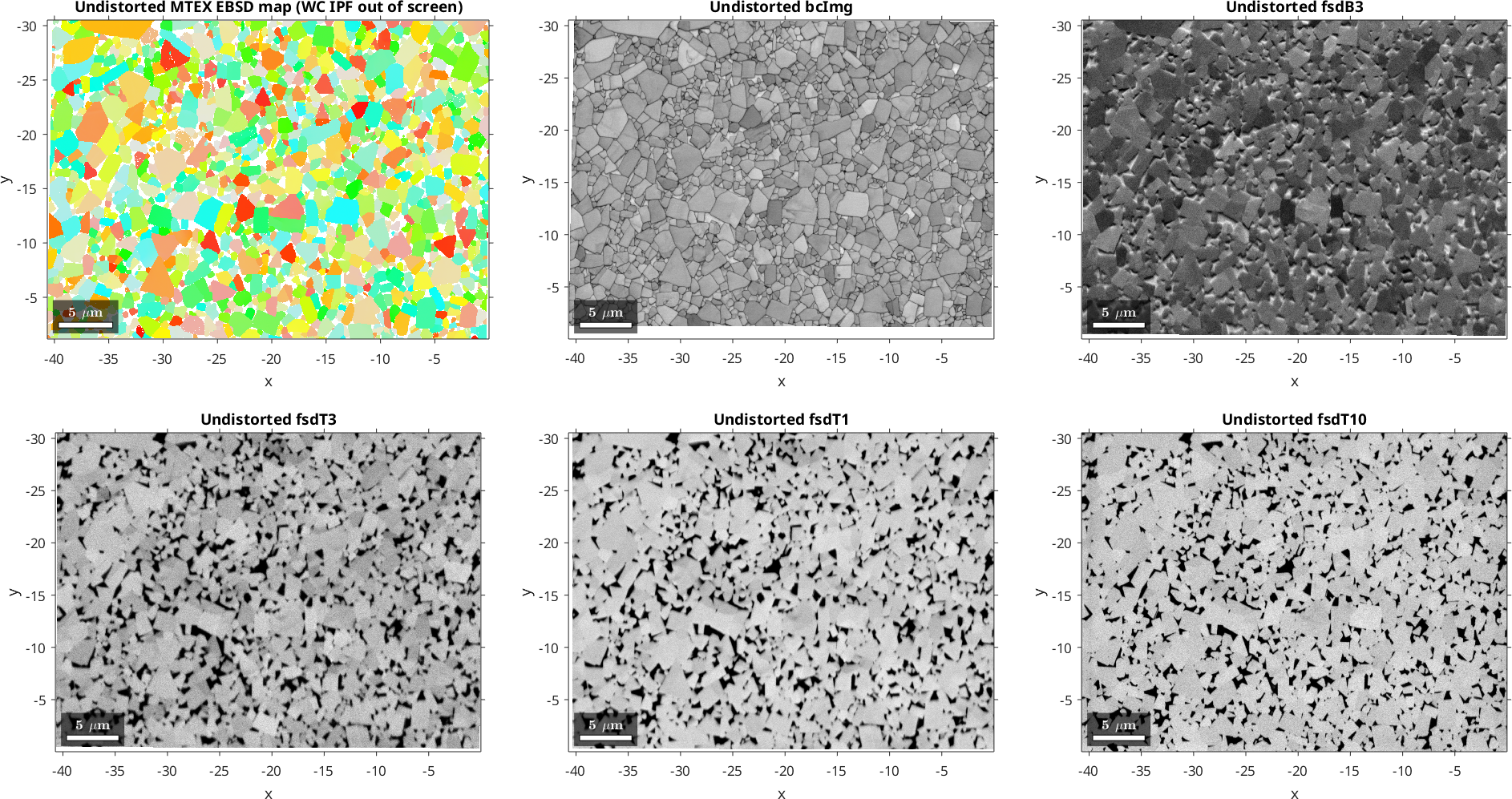
Finish
The map and the images now overlay pixel for pixel, and ebsdOut is an ordinary MTEX EBSD map that happens to carry four SEM images as properties. Anything you would normally do with a map works from here — including turning a thresholded image into a phase, which is what the copper page does with its voids.
For this sample the next step is measuring WC grain contiguity: which boundaries are WC against WC, and which are WC against binder. That needs the orientation data and the image contrast to agree pixel for pixel, which is what the last few minutes bought.
Citing this page.
This page is part of the documentation of
MTEX, a free and open
source MATLAB toolbox for analyzing and modeling crystallographic textures.
It was written by The MTEX Developers and is published at
https://mtex-toolbox.github.io/example_WCCo_2.html.
If you use MTEX, or reuse text or figures from this page, in your research,
please cite
F. Bachmann, R. Hielscher, H. Schaeben: Texture Analysis with MTEX - Free and Open Source Software Toolbox, Solid State Phenomena 160 (2010), 63-68. 10.4028/www.scientific.net/SSP.160.63
BibTeX
@article{bachmann2010mtex,
  author  = {F. Bachmann and R. Hielscher and H. Schaeben},
  title   = {Texture Analysis with MTEX - Free and Open Source Software Toolbox},
  journal = {Solid State Phenomena},
  volume  = {160},
  pages   = {63-68},
  year    = {2010},
  doi     = {10.4028/www.scientific.net/SSP.160.63},
  url     = {https://doi.org/10.4028/www.scientific.net/SSP.160.63}
}
Other papers describing specific MTEX methods are listed under Publications — please cite the one that best fits your application. The MTEX source code is licensed under the GNU General Public License v2.0; the text and figures of this documentation are licensed under CC BY 4.0, which permits reuse — including by automated systems — provided The MTEX Developers and this page are credited.