Lattice Metric and Plane Geometry

Miller indices identify a lattice direction or plane family. The lattice metric supplies the lengths and angles that turn those indices into physical geometry. It determines the length of \([uvw]\), the normal to \((hkl)\), and the spacing between neighbouring \((hkl)\) planes.

In MTEX, a crystalSymmetry bundles point symmetry with a crystal frame. The crystal frame carries the lattice basis and its metric; symmetry states which operations leave crystal data invariant. Keeping those ideas separate matters because a lattice metric can have more symmetry than the atoms placed in its cell.

cs = crystalSymmetry('12/m1',[5.2 6.3 7.1],...
  [90 106 90]*degree,'X||a','mineral','Example monoclinic crystal');

Reading the Lattice Parameters

The three axis lengths and the three interaxial angles are available as abc and abg. MTEX does not attach a unit label to the axis lengths: it preserves the numerical scale supplied by the user or data file. Angstrom is common for crystallographic data, but any consistent length unit works.

cs.abc

ans =
    5.2000    6.3000    7.1000

cs.abg ./ degree

ans =
    90   106    90

The Unit Cell

The unit cell is the parallelepiped spanned by \(\vec a\), \(\vec b\) and \(\vec c\). Repeating it by integer multiples of these three vectors fills the lattice. The cell geometry does not say which atoms or other motif are repeated at its translation points.

The Seven Crystal Systems

A crystal system restricts which lattice parameters may differ. MTEX records the system in cs.lattice and supplies its conventional default angles. The constructor checks required equal axis lengths. For a monoclinic point group, it also checks the two right angles associated with the selected unique axis.

MTEX represents trigonal and hexagonal point groups using the same conventional hexagonal metric; their threefold and sixfold point symmetries distinguish the systems.

The monoclinic point-group symbol also states which axis is unique. The pages on crystal reference frames and axis alignment explain how those lattice axes are placed in MTEX's Cartesian crystal frame.

cs.lattice

ans = 
  latticeType enumeration
    monoclinic

The Reciprocal Basis

Lattice planes are most naturally described in the basis dual to the direct-lattice vectors. If

\[V=\vec a\cdot(\vec b\times\vec c),\]

then

\[\vec a^*=\frac{\vec b\times\vec c}{V},\qquad \vec b^*=\frac{\vec c\times\vec a}{V},\qquad \vec c^*=\frac{\vec a\times\vec b}{V}.\]

The direct and reciprocal bases are dual: each direct axis has dot product one with its matching reciprocal axis and zero with the other two. MTEX provides them as axes and axesDual.

directBasis = cs.axes;
reciprocalBasis = cs.axesDual;

cellVolume = abs(det(directBasis))

cellVolume =
  223.5856

The output is 223.5856 in the cube of the lattice-parameter unit. The defining duality is seen directly in the matrix of pairwise dot products.

dot_outer(directBasis,reciprocalBasis)

ans =
    1.0000         0         0
    0.0000    1.0000         0
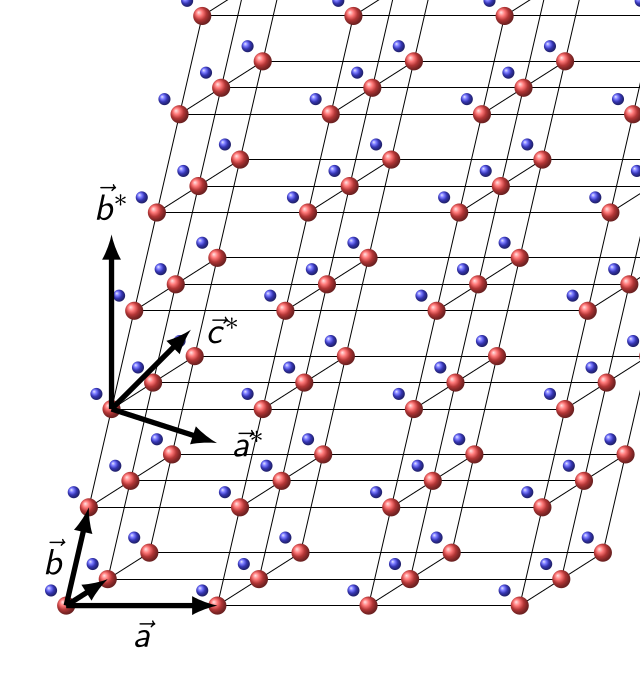
    0.0000    0.0000    1.0000

The result is the identity matrix. Reciprocal axes have inverse-length units, and MTEX uses the crystallographic convention without a factor \(2\pi\). Direct and reciprocal axes are parallel in an orthogonal lattice; in a monoclinic or triclinic lattice they generally are not.

The schematic shows the direct basis at the lower left and the reciprocal basis from a second lattice point. The red points are translation-equivalent positions, while the blue points illustrate a repeated motif. Notice in particular that \(\vec a\) and \(\vec a^*\) are not parallel.

Lengths of Lattice Directions

A direct-lattice direction is a real vector

\[\vec m=u\vec a+v\vec b+w\vec c.\]

Its norm is therefore a physical length, not just a plotting radius. The indices are coefficients in the generally oblique lattice basis, not Cartesian components. For example, \([101]\) spans one \(\vec a\) and one \(\vec c\).

m = Miller(1,0,1,cs,'uvw');

norm(m)

ans =
    7.5563

The value 7.5563 is in the same units as cs.abc. Multiplying all indices by two leaves the geometric direction unchanged, up to numerical rounding, but doubles the vector length. The option 'noSymmetry' compares the two vectors as written rather than searching their symmetry-equivalent directions.

angle(m,Miller(2,0,2,cs,'uvw'),'noSymmetry') ./ degree

ans =
   8.5377e-07

norm(Miller(2,0,2,cs,'uvw')) ./ norm(m)

ans =
     2

The angle is numerically zero, while the length ratio is 2.

Use normalize when only the direction matters. Keep the original magnitude when the lattice translation or Burgers-vector length is part of the calculation.

Interplanar Spacing

The normal of \((hkl)\) is a reciprocal-lattice vector. MTEX uses the crystallographic convention without a factor \(2\pi\), so its length is the inverse of the interplanar spacing returned by dspacing:

\[ d_{hkl}=\frac{1}{\lVert\vec n_{hkl}\rVert}. \]

h = Miller(1,0,0,cs);

d100 = dspacing(h)

d100 =
    4.9986

MTEX returns 4.9986, which is smaller than \(a=5.2\). In this monoclinic cell, \(\vec a\) is not perpendicular to the \((100)\) planes. The spacing is the component of \(\vec a\) normal to those planes, not generally the length of \(\vec a\).

The same command works for a list. For a cubic lattice with parameter \(a=3.6\), the familiar result is \(d_{hkl}=a/\sqrt{h^2+k^2+l^2}\).

csCubic = crystalSymmetry('m-3m',[3.6 3.6 3.6]);
hCubic = Miller({1,0,0},{1,1,0},{1,1,1},csCubic);

dspacing(hCubic)

ans =
    3.6000    2.5456    2.0785

The \((100)\), \((110)\), and \((111)\) spacings are 3.6000, 2.5456, and 2.0785. In a cubic lattice the spacing decreases as the squared-index sum \(h^2+k^2+l^2\) increases.

The Maths Behind the Metric

Put the direct-basis vectors into \(A=[\vec a\ \vec b\ \vec c]\). The metric matrix is the matrix of their pairwise dot products,

\[G=A^{\mathrm T}A,\qquad G_{ij}=\vec a_i\mathbin{\cdot}\vec a_j.\]

MTEX obtains it directly from the basis vectors.

metricMatrix = dot_outer(directBasis,directBasis)

metricMatrix =
   27.0400    0.0000  -10.1765
    0.0000   39.6900    0.0000
  -10.1765    0.0000   50.4100

The diagonal entries are \(a^2\), \(b^2\), and \(c^2\). The off-diagonal entries contain the interaxial angles, so the nonzero \(a\) -- \(c\) terms record the monoclinic angle \(\beta=106^\circ\).

For the direct-index column \(\mathbf u=(u,v,w)^{\mathrm T}\) and the reciprocal-index column \(\mathbf h=(h,k,l)^{\mathrm T}\),

\[\lVert\vec m\rVert^2=\mathbf u^{\mathrm T}G\mathbf u, \qquad G^*=G^{-1},\qquad d_{hkl}=\frac{1}{\sqrt{\mathbf h^{\mathrm T}G^*\mathbf h}}.\]

These equations are the matrix form of the norm and dspacing calculations above. They also give \(V=\sqrt{\det G}\) for the unit-cell volume.

What a Crystal Symmetry Does Not Store

The crystal geometry used here contains point symmetry and a crystal frame with its lattice metric. It does not model an atomic basis, Wyckoff positions, or the translational parts of a space group. In particular, the 14 Bravais lattices distinguish translational centring, whereas crystalSymmetry retains the associated crystal system and point group.

A CIF can supply lattice parameters and a space-group symbol. When MTEX constructs a crystalSymmetry from that information, it reduces the space group to its point group for this geometry. Structure factors and systematic absences therefore require information outside this model.

References

Next

Operations uses direct and reciprocal geometry for incidence tests, zone axes, angles, and multiplicities. Reference System explains how the lattice basis is embedded in a Cartesian crystal frame.