Pole Figure Tutorial

Tutorial on x-ray and neutron diffraction data.

Import diffraction data

Click on Import pole figure data to start the import wizard which is a GUI leading you through the import of pole figure data. After finishing the wizard you will end with a script similar to the following one.

% This script was automatically created by the import wizard. You should
% run the whole script or parts of it in order to import your data. There
% is no problem in making any changes to this script.

% *Specify Crystal and Specimen Symmetries*

% crystal symmetry
CS = crystalSymmetry('6/mmm', [2.633 2.633 4.8], 'X||a*', 'Y||b', 'Z||c');

% specimen symmetry
SS = specimenSymmetry('1');

% plotting convention
setMTEXpref('xAxisDirection','north');
setMTEXpref('zAxisDirection','outOfPlane');

% *Specify File Names*

% path to files
pname = [mtexDataPath filesep 'PoleFigure' filesep 'ZnCuTi' filesep];

% which files to be imported
fname = {...
  [pname 'ZnCuTi_Wal_50_5x5_PF_002_R.UXD'],...
  [pname 'ZnCuTi_Wal_50_5x5_PF_100_R.UXD'],...
  [pname 'ZnCuTi_Wal_50_5x5_PF_101_R.UXD'],...
  [pname 'ZnCuTi_Wal_50_5x5_PF_102_R.UXD'],...
  };

% defocusing
fname_def = {...
  [pname 'ZnCuTi_defocusing_PF_002_R.UXD'],...
  [pname 'ZnCuTi_defocusing_PF_100_R.UXD'],...
  [pname 'ZnCuTi_defocusing_PF_101_R.UXD'],...
  [pname 'ZnCuTi_defocusing_PF_102_R.UXD'],...
  };

% *Specify Miller Indices*

h = { ...
  Miller(0,0,2,CS),...
  Miller(1,0,0,CS),...
  Miller(1,0,1,CS),...
  Miller(1,0,2,CS),...
  };

% *Import the Data*

% create a Pole Figure variable containing the data
pf = PoleFigure.load(fname,h,CS,SS,'interface','uxd');

% defocusing
pf_def = PoleFigure.load(fname_def,h,CS,SS,'interface','uxd');

% correct data
pf = correct(pf,'def',pf_def);

Plot Raw Data

You should run the script section wise to see how MTEX imports the pole figure data. Next, you can plot your data

plot(pf)

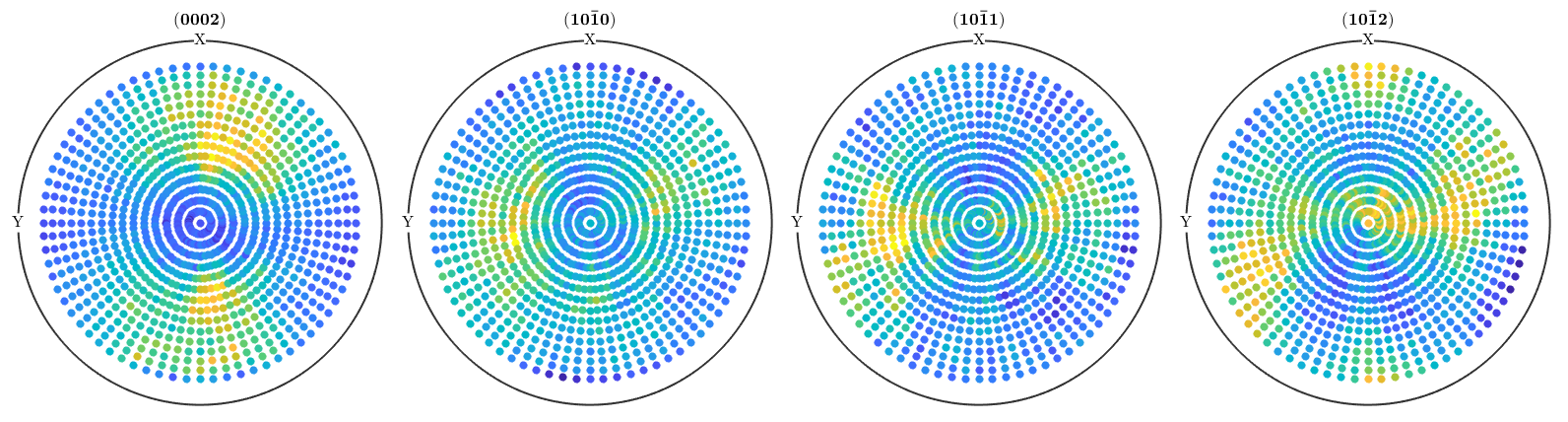
Make sure that the Miller indices are correctly assigned to the pole figures and that the alignment of the specimen coordinate system, i.e., X, Y, Z is correct. In case of outliers or misaligned data, you may want to correct your raw data. See how to modify pole figure data for further information.

ODF Estimation

Once your data are in a good shape, i.e. defocusing correction has been done and only few outliers are left you can stop to reconstruct an ODF out of these data. This is done by the command calcODF.

odf = calcODF(pf,'silent')

 
odf = ODF  
  crystal symmetry : 6/mmm, X||a*, Y||b, Z||c*
  specimen symmetry: 1
 
  Uniform portion:
    weight: 0.53416
 
  Radially symmetric portion:
    kernel: de la Vallee Poussin, halfwidth 10°
    center: 9922 orientations, resolution: 5°
    weight: 0.46584

Note that reconstructing an ODF from pole figure data is a severely ill- posed problem, i.e., it does not provide a unique solution. A more throughout the discussion on the ambiguity of ODF reconstruction from pole figure data can be found here. As a rule of thumb: as more pole figures you have and as more consistent you pole figure data are as better you reconstructed ODF will be.

To check how well your reconstructed ODF fits the measured pole figure data do

plotPDF(odf,pf.h)

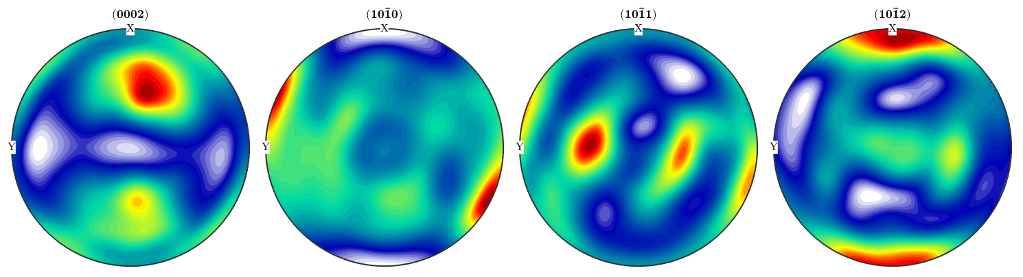
Compare the recalculated pole figures with the measured data. A quantitative measure for the fitting are the so called RP values. They can be computed by

calcError(odf,pf)

progress: 100%
ans =
    0.0556    0.0450    0.0609    0.0444

In the case of a bad fitting, you may want to tweak the reconstruction algorithm. See here for more information.

Quantify the Reconstruction Error

Visualize the ODF

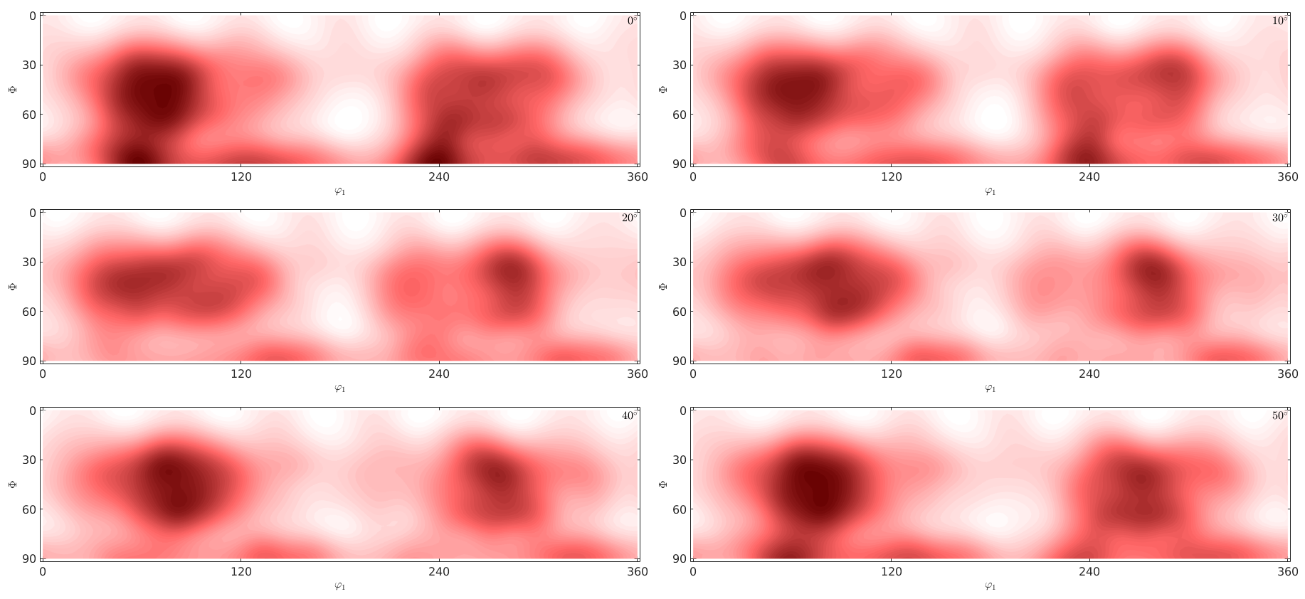
plot(odf)
mtexColorMap LaboTeX

progress: 100%

restore old setting

setMTEXpref('xAxisDirection','east');