Modify Pole Figure Data

Import diffraction data

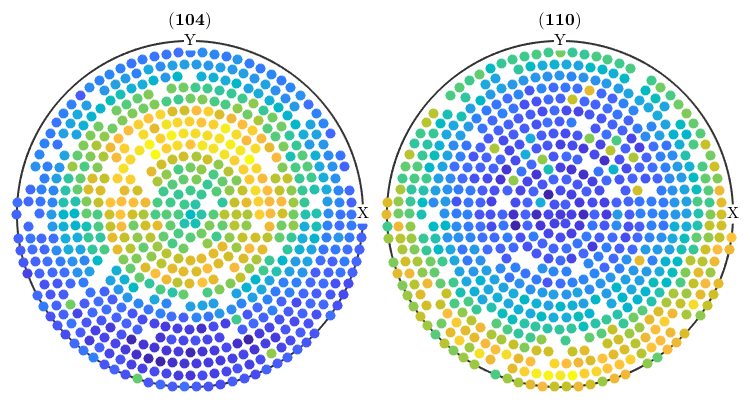
Let us load some data and plot them.

mtexdata geesthacht

% plot imported polefigure
plot(pf)

 loading data ...
 saving data to /home/hielscher/mtex/master/data/geesthacht.mat

Back to Top

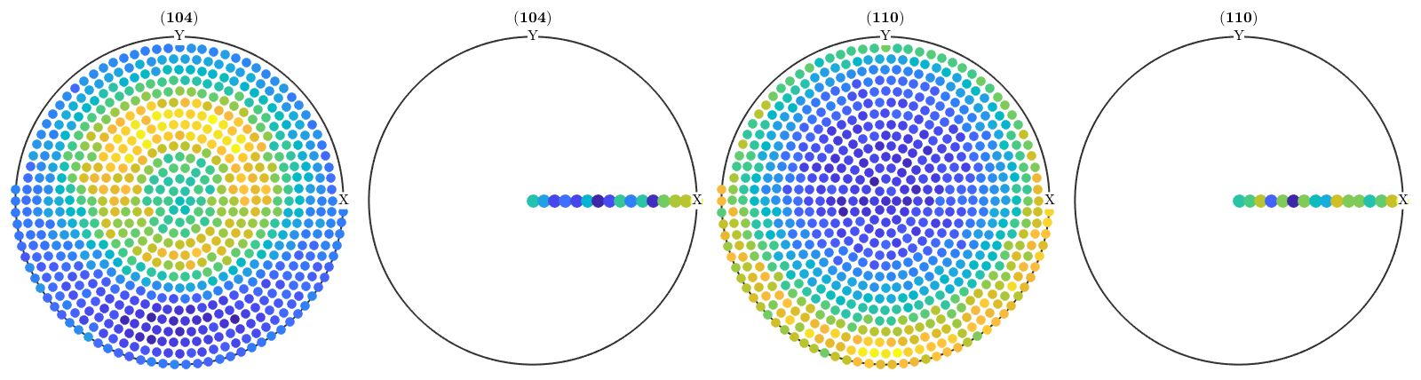
Splitting and Reordering of Pole Figures

As we can see the first and the third pole figure complete pole figures and the second and the fourth pole figures contain some values for background correction. Let us, therefore, split the pole figures into these two groups.

pf_complete = pf({1,3})
pf_background= pf({2,4})

 
pf_complete = PoleFigure  
  crystal symmetry : m-3m
  specimen symmetry: -1
 
  h = (104), r = 679 x 1 points
  h = (110), r = 679 x 1 points
 
pf_background = PoleFigure  
  crystal symmetry : m-3m
  specimen symmetry: -1
 
  h = (104), r = 16 x 1 points
  h = (110), r = 16 x 1 points

Actually, it is possible to work with pole figures as with simple numbers. E.g. it is possible to add / subtract pole figures. A superposition of the first and the third pole figures can be written as

2*pf({1}) + 3*pf({3})

 
ans = PoleFigure  
  crystal symmetry : m-3m
  specimen symmetry: -1
 
  h = (104)(110), r = 679 x 1 points

Back to Top

Correct pole figure data

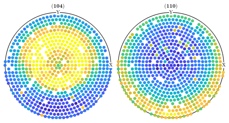
In order to correct pole figures for background radiation and defocusing one can use the command correct. In our case the syntax is

pf = correct(pf_complete,'background',pf_background);
plot(pf)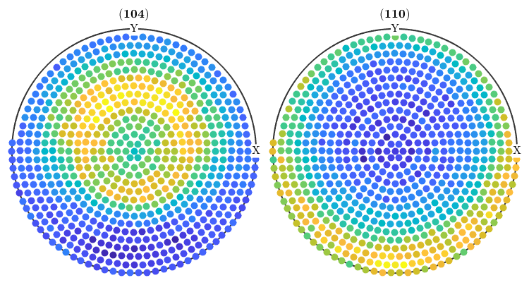

Back to Top

Normalize pole figures

Sometimes people want to have normalized pole figures. In the case of complete pole figures, this can be simply archived using the command normalize

pf_normalized = normalize(pf);
plot(pf_normalized)

However, in the case of incomplete pole figures, it is well known, that the normalization can only by computed from an ODF. Therefore, one has to proceed as follows:

% compute an ODF from the pole figure data
odf = calcODF(pf);

% and use it for normalization
pf_normalized = normalize(pf,odf);

plot(pf_normalized)

Back to Top

Modify certain pole figure values

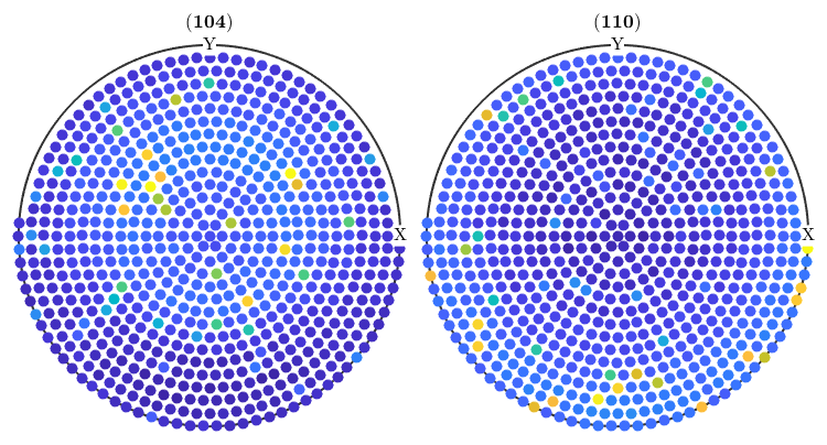
As pole figures are usually experimental data they may contain outliers. In order to remove outliers from pole figure data one can use the function isOutlier. Here a simple example:

% Let us add 100 random outliers to the pole figure data
% First we select 100 random positions within the pole figures
ind = randperm(pf.length,100);

% Next we multiply the intensity at these positions by a random value
% between 3 and 4
factor = 3+rand(100,1);
pf(ind).intensities = pf(ind).intensities(:) .* factor;

% Let's check the result
plot(pf)

check for outliers

condition = pf.isOutlier;

% remove outliers
pf(condition) = [];

% plot the corrected pole figures
plot(pf)

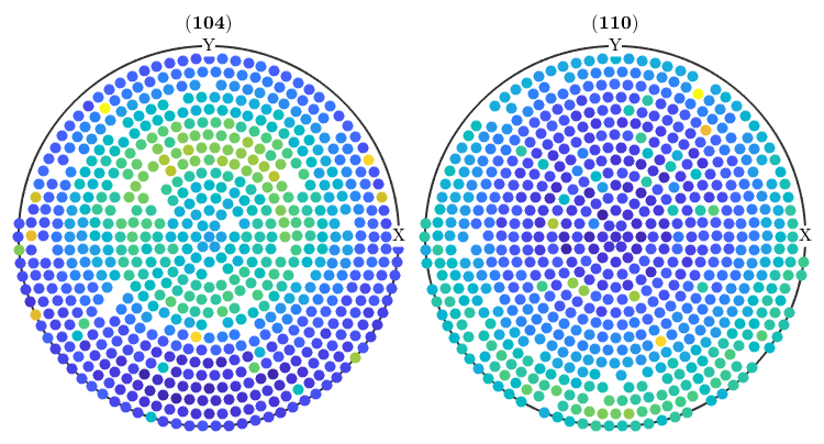
Sometimes applying the above correction is not suffcient. Then it can help to repeat the outlier detection ones again

pf(pf.isOutlier) = [];
plot(pf)

Back to Top

Remove certain measurements from the data

In the same way, as we removed the outlier one can manipulate and delete pole figure data by any criteria. Lets, e.g. cap all values that are larger than 500.

% find those values
condition = pf.intensities > 500;

% cap the values in the pole figures
pf(condition).intensities = 500;

plot(pf)

Back to Top

Rotate pole figures

Sometimes it is necessary to rotate the pole figures. In order to do this with MTEX one has first to define a rotation, e.e. by

% This defines a rotation around the x-axis about 100 degree
rot = rotation.byAxisAngle(xvector,100*degree);

Second, the command rotate can be used to rotate the pole figure data.

pf_rotated = rotate(pf,rot);
plot(pf_rotated,'antipodal')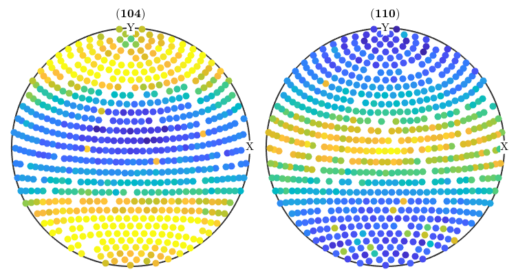

Back to Top

DocHelp 0.1 beta