Ambiguity of the Pole Figure to ODF Reconstruction Problem
demonstrates different sources of ambiguity when reconstructing an ODF from pole figure diffraction data.
| On this page ... |
| The ambiguity due to too few pole figures |
| The ambiguity due to too Friedel's law |
| The inherent ambiguity of the pole figure - ODF relationship |
The ambiguity due to too few pole figures
Due to experimental limitations, one is usually restricted to a short list of crystal directions (Miller indices) for which diffraction pole figures can be measured. In general, more measured pole figures implies more reliable ODF reconstruction and low-symmetry materials and weak textures usually requires more pole figures then sharp texture with a high crystal symmetry. From a theoretical point of view, the number of pole figures should be at a level with the square root of the number of pole points in each pole figure. This is of course far from experimentally possible.
Let's demonstrate the ambiguity due to too few pole figures at the example of two orthorhombic ODFs. The first ODF has three modes at the positions
cs = crystalSymmetry('mmm');

orix = orientation.byAxisAngle(xvector,90*degree,cs);
oriy = orientation.byAxisAngle(yvector,90*degree,cs);
oriz = orientation.byAxisAngle(zvector,90*degree,cs);

odf1 = unimodalODF([orix,oriy,oriz])
odf1 = ODF
  crystal symmetry : mmm
  specimen symmetry: 1

  Radially symmetric portion:
    kernel: de la Vallee Poussin, halfwidth 10°
    center: Rotations: 1x3
    weight: 1
The second ODF has three modes as well but this times at rotations about the axis (1,1,1) with angles 0, 120, and 240 degrees.
ori = orientation.byAxisAngle(vector3d(1,1,1),[0,120,240]*degree,cs);
odf2 = unimodalODF(ori)
odf2 = ODF
  crystal symmetry : mmm
  specimen symmetry: 1

  Radially symmetric portion:
    kernel: de la Vallee Poussin, halfwidth 10°
    center: Rotations: 1x3
    weight: 1
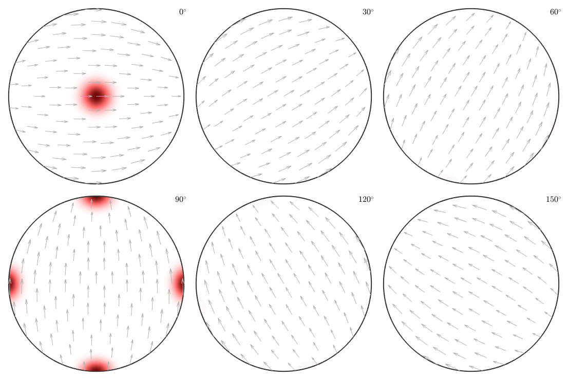
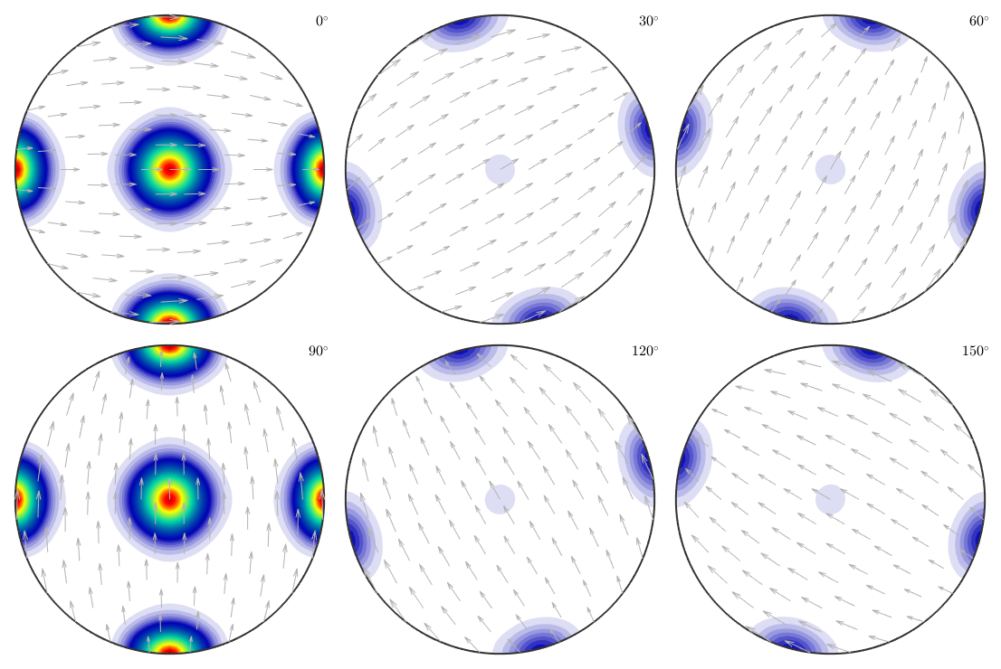
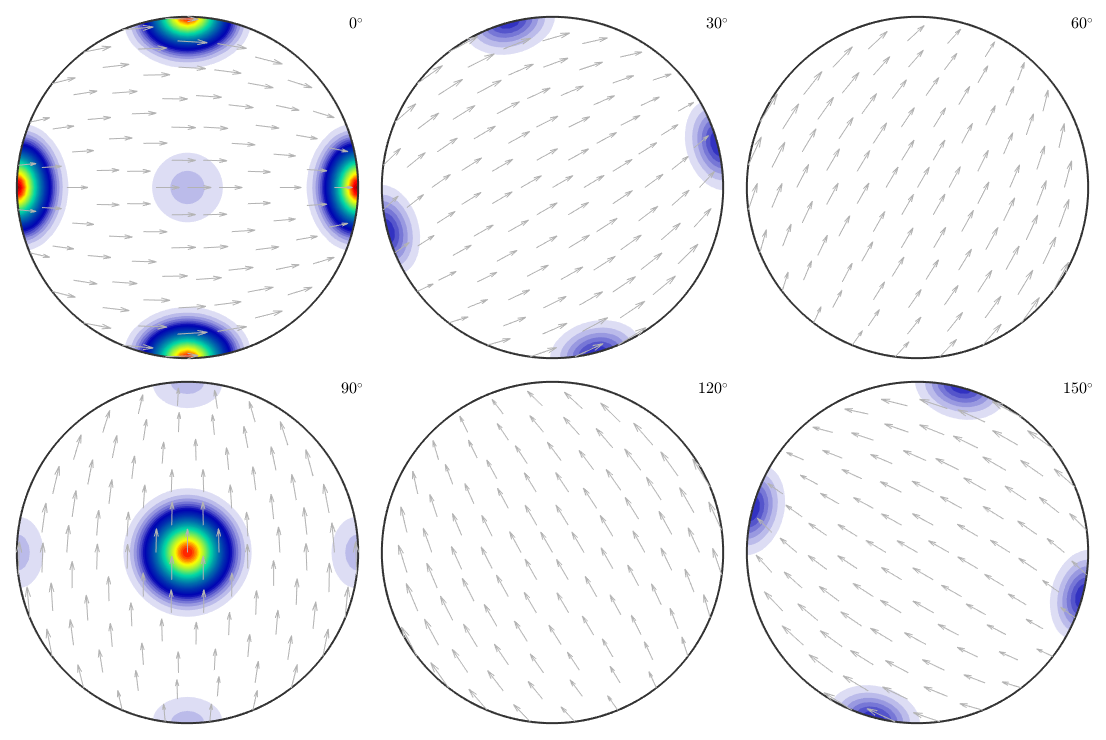
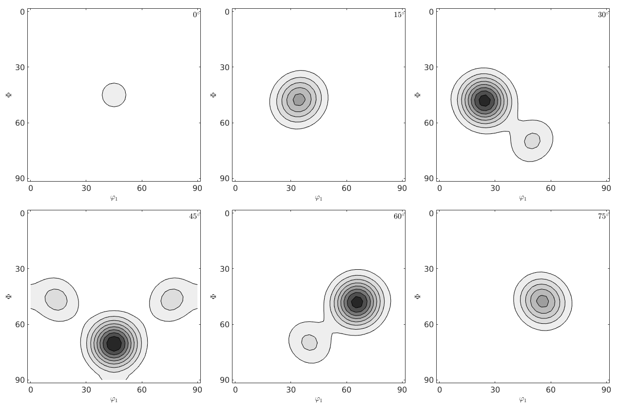
These two ODFs are completely disjoint. Let's check this by plotting them as sigma sections
figure(1)
plot(odf1,'sigma')
mtexColorMap LaboTeX
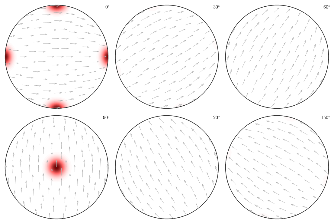
figure(2)
plot(odf2,'sigma')
mtexColorMap LaboTeX
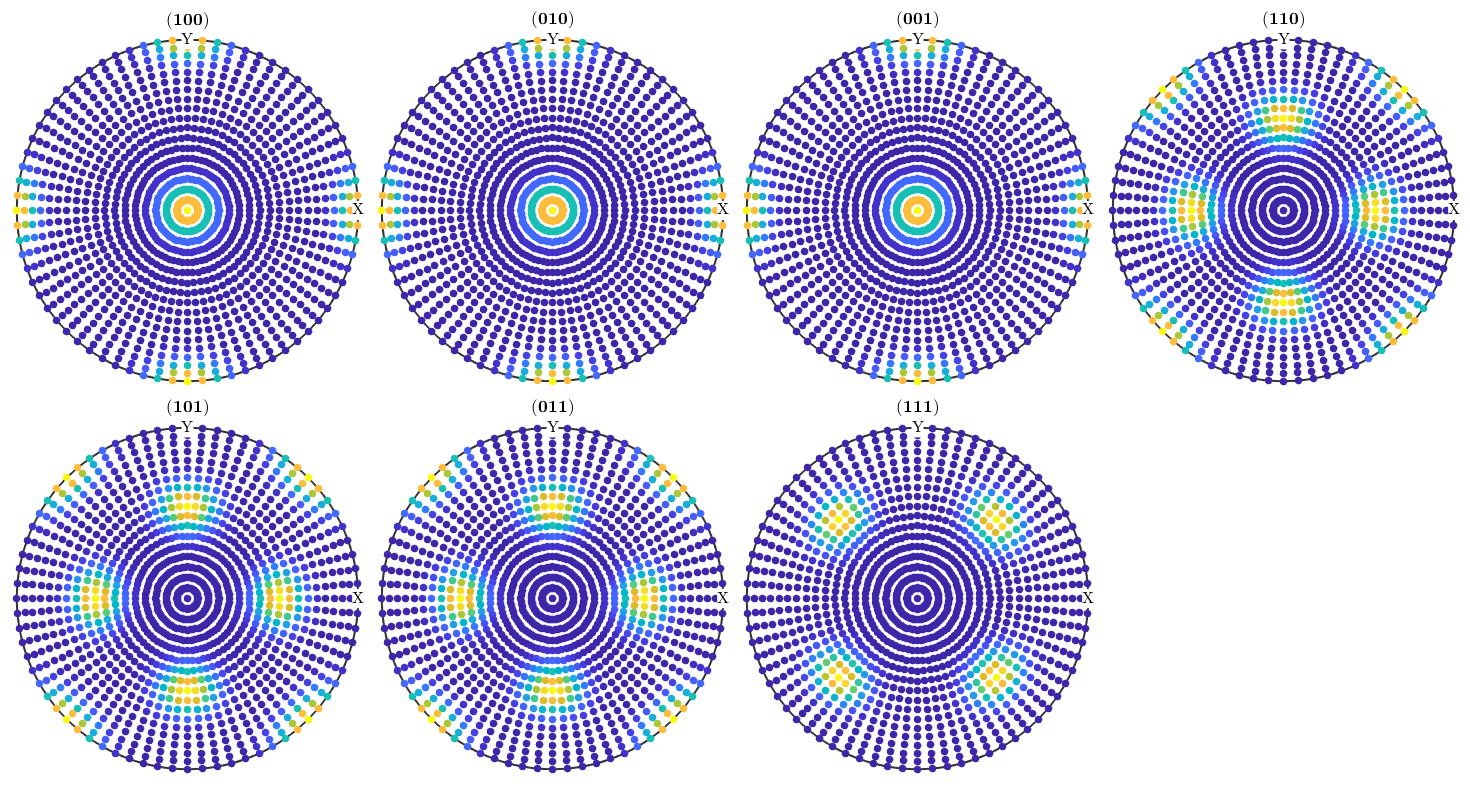
However, when it comes to pole figures 7 of them, namely, (100), (010), (001), (110), (101), (011) and (111), are identical for both ODFs. Of course looking at any other pole figure makes clear that those two ODFs are different.
figure(1)
h = Miller({1,0,0},{0,1,0},{0,0,1},{1,1,0},{1,0,1},{0,1,1},{1,1,1},{1,2,0},cs);
plotPDF(odf1,h,'contourf')
mtexColorMap LaboTeX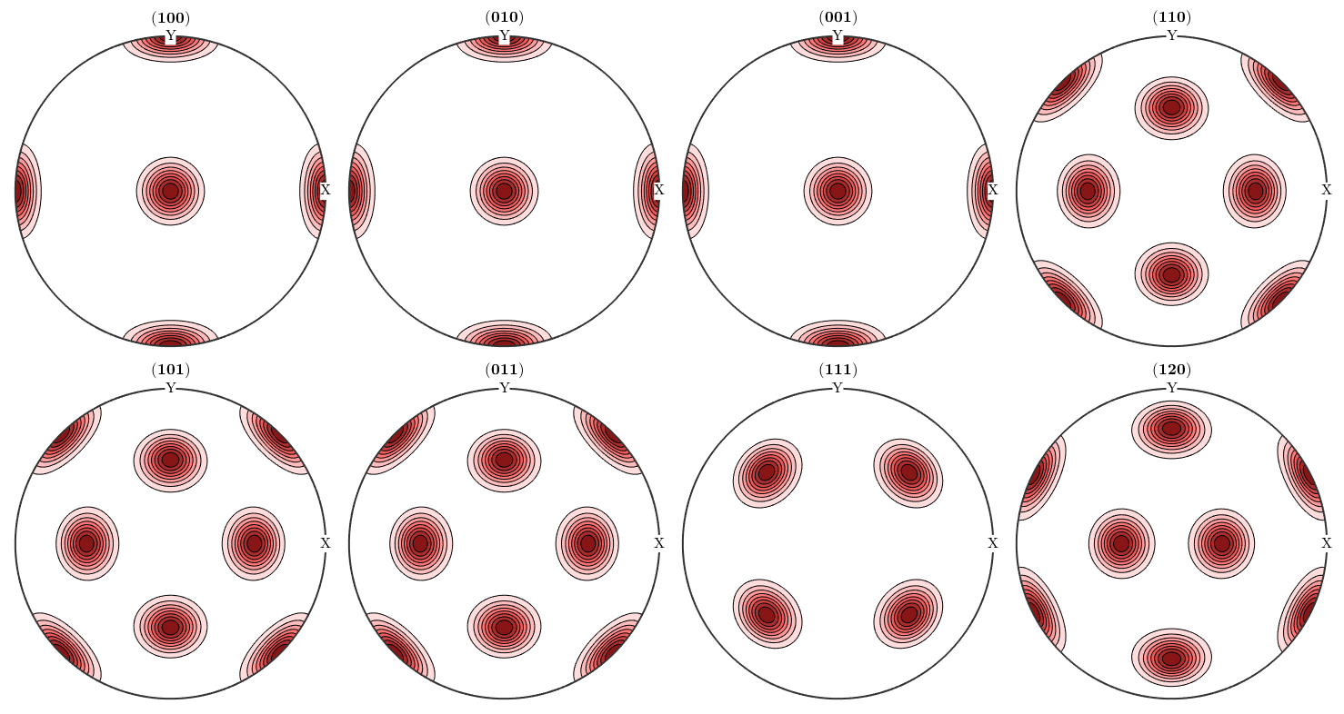
figure(2)
plotPDF(odf2,h,'contourf')
mtexColorMap LaboTeX
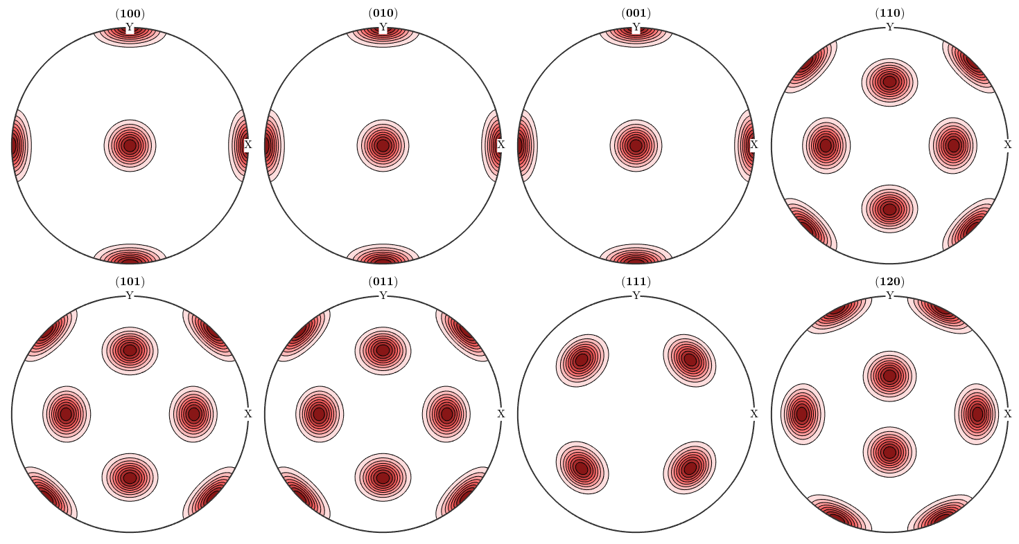
The question is now, how can any pole figure to ODF reconstruction algorithm decide which of the two ODFs was the true one if only the seven identical pole figures (100), (010), (001), (110), (101), (011), (111) have been measured? The answer is: this is impossible to decide. Next question is: which result will I get from the MTEX reconstruction algorithm? Let's check this
% 1. step: simulate pole figure data
pf = calcPoleFigure(odf1,h(1:7),'upper');

plot(pf)
2. step: reconstruct an ODF
odf = calcODF(pf,'silent')

plot(odf,'sigma')
odf = ODF
  crystal symmetry : mmm
  specimen symmetry: 1

  Radially symmetric portion:
    kernel: de la Vallee Poussin, halfwidth 10°
    center: 29765 orientations, resolution: 5°
    weight: 1

progress: 100%
We observe that the reconstructed ODF is an almost perfect mixture of the first and the second ODF. Actually, any mixture of the two initial ODFs would have been a correct answer. However, the ODF reconstructed by the MTEX algorithm can be seen as the ODF which is closest to the uniform distribution among all admissible ODFs.
Finally, we increase the number of pole figures by five more crystal directions and perform our previous experiment once again.
% 1. step: simulate pole figure data for all crystal directions
h = [h,Miller({0,1,2},{2,0,1},{2,1,0},{0,2,1},{1,0,2},cs)];
pf = calcPoleFigure(odf1,h,'upper');

% 2. step: reconstruct an ODF
odf = calcODF(pf,'silent')

plot(odf,'sigma')
odf = ODF
  crystal symmetry : mmm
  specimen symmetry: 1

  Radially symmetric portion:
    kernel: de la Vallee Poussin, halfwidth 10°
    center: 29763 orientations, resolution: 5°
    weight: 1

progress: 100%
Though the components of odf2 are still present in the recalculated ODF they are far less pronounced compared to the components of odf1.
% 1. step: simulate pole figure data for all crystal directions
pf = calcPoleFigure(odf1,h,'upper');

% 2. step: reconstruct an ODF
odf = calcODF(pf,'silent')

plot(odf,'sigma')
odf = ODF
  crystal symmetry : mmm
  specimen symmetry: 1

  Radially symmetric portion:
    kernel: de la Vallee Poussin, halfwidth 10°
    center: 29763 orientations, resolution: 5°
    weight: 1

progress: 100%

The ambiguity due to too Friedel's law
Due to Friedel's law pole figure data always impose antipodal symmetry. In order to demonstrate the consequences of this antipodal symmetry we consider crystal symmetry -43m
cs = crystalSymmetry('-43m')cs = crystalSymmetry symmetry: -43m a, b, c : 1, 1, 1
and two rotations
ori1 = orientation.byEuler(30*degree,60*degree,10*degree,cs)
ori2 = orientation.byEuler(30*degree,60*degree,100*degree,cs)
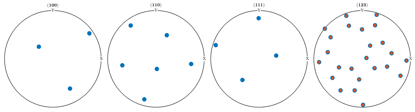
h = Miller({1,0,0},{1,1,0},{1,1,1},{1,2,3},cs);
plotPDF(ori1,h,'MarkerSize',12)
hold on
plotPDF(ori2,'MarkerSize',8)
hold off
ori1 = orientation
  size: 1 x 1
  crystal symmetry : -43m
  specimen symmetry: 1

  Bunge Euler angles in degree
  phi1  Phi phi2 Inv.
    30   60   10    0


ori2 = orientation
  size: 1 x 1
  crystal symmetry : -43m
  specimen symmetry: 1

  Bunge Euler angles in degree
  phi1  Phi phi2 Inv.
    30   60  100    0
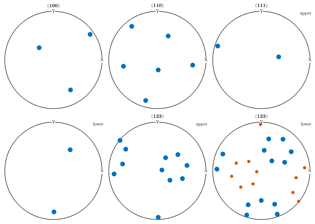
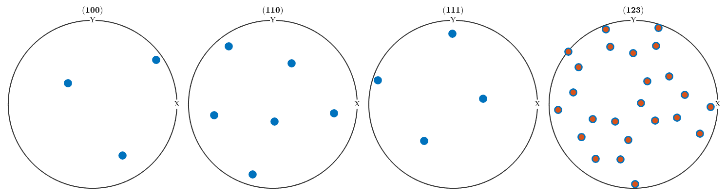
Obviously, both orientations are not symmetrically equivalent as -43m does not have a four fold axis. This can also be seen from the pole figure plots above which are different for, e.g., (111). However, when looking at an arbitrary pole figure with additionaly imposed antipodal symmetry both orientations appears at exactly the same positions
plotPDF(ori1,h,'MarkerSize',12,'antipodal')
hold on
plotPDF(ori2,'MarkerSize',8)
hold off
The reason is that adding antipodal symmetry to all pole figures is equivalent to adding the inversion as an additional symmetry to the point group, i.e., to replace it by the Laue group. Which is illustrated in the following plot
ori1.CS= ori1.CS.Laue;
ori2.CS= ori2.CS.Laue;
h.CS = h.CS.Laue;

plotPDF(ori1,h,'MarkerSize',12)
hold on
plotPDF(ori2,'MarkerSize',8)
hold off
As a consequence of Friedels law, all noncentrosymmetric information about the texture is lost in the diffraction pole figures and we can only aim at recovering the centrosymmetric portion. In particular, any ODF that is reconstructed by MTEX from diffraction pole figures is centrosymmetric, i.e. its point group is a Laue group. If the point group of the crystal was already a Laue group then Fridel's law does not impose any additional ambiguity.
The inherent ambiguity of the pole figure - ODF relationship
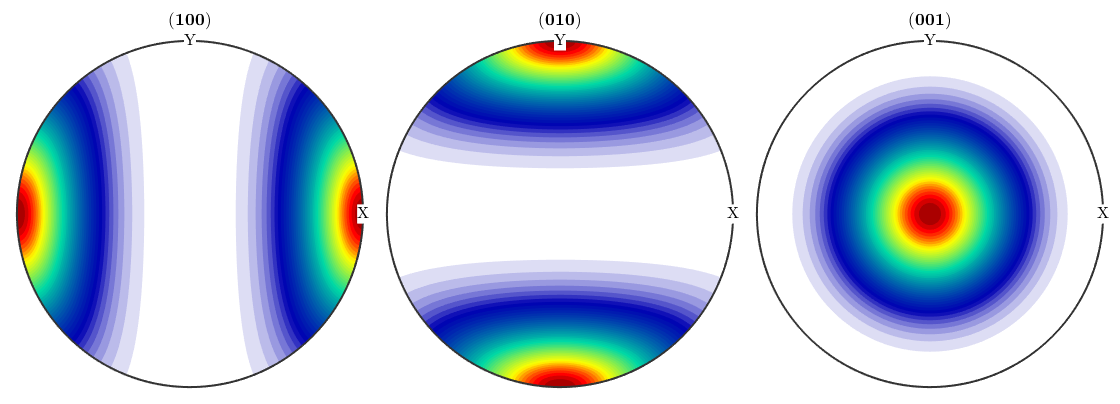
Unfortunately, knowing all diffraction pole figures of an ODF is even for centrosymmetric symmetries not sufficient to recover the ODF unambiguously. To understand the reason for this ambiguity we consider triclinic symmetry and a week unimodal ODF with prefered orientation (0,0,0).
cs = crystalSymmetry('-1');

odf1 = 2/3 * uniformODF(cs) + 1/3 * unimodalODF(orientation.id(cs),'halfwidth',30*degree)

plotPDF(odf1,Miller({1,0,0},{0,1,0},{0,0,1},cs),'antipodal')
odf1 = ODF
  crystal symmetry : -1, X||a, Y||b*, Z||c*
  specimen symmetry: 1

  Uniform portion:
    weight: 0.66667

  Radially symmetric portion:
    kernel: de la Vallee Poussin, halfwidth 30°
    center: (0°,0°,0°)
    weight: 0.33333
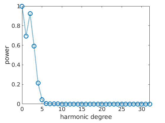
As any other ODF, we can represent it by its series expansion by harmonic functions. This does not change the ODF but only its representation
odf1 = FourierODF(odf1,10)

plotPDF(odf1,Miller({1,0,0},{0,1,0},{0,0,1},cs))
odf1 = ODF
  crystal symmetry : -1, X||a, Y||b*, Z||c*
  specimen symmetry: 1
  antipodal:         true

  Harmonic portion:
    degree: 9
    weight: 1

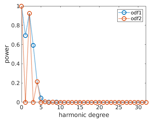
We may look at the coefficients of this expansion and observe how the decay to zero rapidly. This justifies to cut the harmonic expansion at harmonic degree 10.
close all
plotFourier(odf1,'linewidth',2)
%set(gca,'yScale','log')
Next, we define a second ODF which differs by the first one only in the odd order harmonic coefficients. More precisely, we set all odd order harmonic coefficients to zero
A = mod(1:11,2);
odf2 = conv(odf1,A)

hold on
plotFourier(odf2,'linewidth',2)
%set(gca,'yScale','log')
hold off
legend('odf1','odf2')
odf2 = ODF
  crystal symmetry : -1, X||a, Y||b*, Z||c*
  specimen symmetry: 1
  antipodal:         true

  Harmonic portion:
    degree: 9
    weight: 1
The point is that all pole figures of odf1 look exactly the same as the pole figures of odf2.
plotPDF(odf2,Miller({1,0,0},{0,1,0},{0,0,1},cs),'antipodal')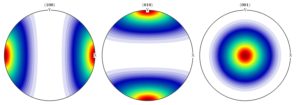
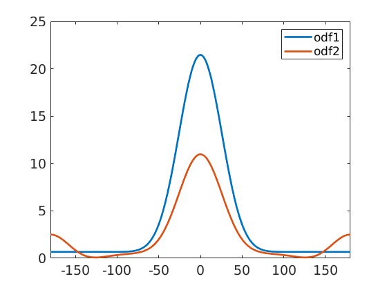
and hence, it is impossible for any reconstruction algorithm to decide whether odf1 or odf2 is the correct reconstruction. In order to compare odf1 and odf2, we visualize them along the alpha fibre
alphaFibre = orientation.byAxisAngle(zvector,(-180:180)*degree,cs);

close all
plot(-180:180,odf1.eval(alphaFibre),'linewidth',2)
hold on
plot(-180:180,odf2.eval(alphaFibre),'linewidth',2)
hold off
legend('odf1','odf2')
xlim([-180,180])
We can make the example more extreme by applying negative coefficients to the odd order harmonic coefficients.
odf1 = 4/5 * uniformODF(cs) + 1/5 * unimodalODF(orientation.id(cs),'halfwidth',30*degree);

A = (-1).^(0:10);
odf2 = conv(odf1,A);

close all
plot(-180:180,odf1.eval(alphaFibre),'linewidth',2)
hold on
plot(-180:180,odf2.eval(alphaFibre),'linewidth',2)
hold off
legend('odf1','odf2')
xlim([-180,180])
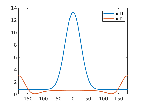
We obtain two completely different ODF: odf1 has a prefered orientation at (0,0,0) while odf2 has prefered orientations at all rotations about 180 degrees. These two ODFs have completely identical pole figures and hence, it is impossible by any reconstruction method to decide which of these two ODF was the correct one. It was the idea of Matthies to say that a physical meaningful ODF usually consists of a uniform portion and some components of prefered orientations. Thus in the reconstruction odf1 should be prefered over odf2. The idea to distinguish between odf1 and odf2 is that odf1 has a larger uniform portion and hence maximizing the uniform portion can be used as a method to single out a physical meaningful solution.
Let's demonstrate this by the given example and simulate some pole figures out of odf2.
h = Miller({1,0,0},{1,0,0},{0,1,0},{0,0,1},{1,1,0},{0,1,1},{1,0,1},{1,1,1},cs);
pf = calcPoleFigure(odf1,h);

plot(pf)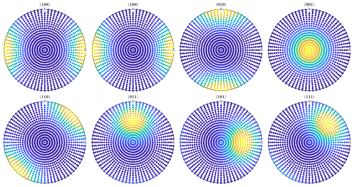
When reconstruction an ODF from pole figure data MTEX automatically uses Matthies methods of maximizing the uniform portion called automatic ghost correction
odf_rec1 = calcODF(pf,'silent')
odf_rec1 = ODF
  crystal symmetry : -1, X||a, Y||b*, Z||c*
  specimen symmetry: 1

  Uniform portion:
    weight: 0.79845

  Radially symmetric portion:
    kernel: de la Vallee Poussin, halfwidth 10°
    center: 118599 orientations, resolution: 5°
    weight: 0.20155
This method can be switched off by the following command
odf_rec2 = calcODF(pf,'noGhostCorrection','silent')
odf_rec2 = ODF
  crystal symmetry : -1, X||a, Y||b*, Z||c*
  specimen symmetry: 1

  Radially symmetric portion:
    kernel: de la Vallee Poussin, halfwidth 10°
    center: 119087 orientations, resolution: 5°
    weight: 1
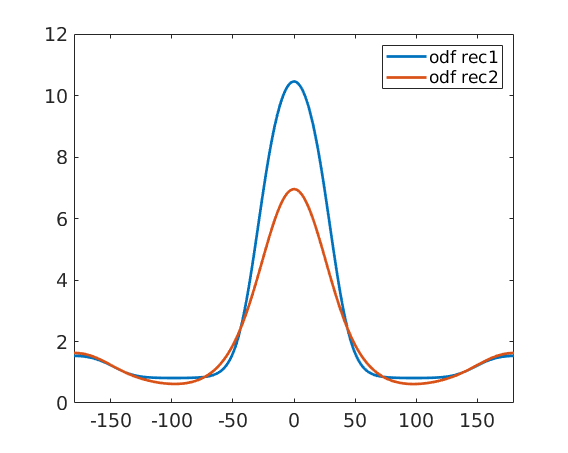
When comparing the reconstructed ODFs we observe that by using ghost correction we are able to recover odf1 quite nicely, while without ghost correction we obtain a mixture between odf1 and odf2.
close all
plot(-180:180,odf_rec1.eval(alphaFibre),'linewidth',2)
hold on
plot(-180:180,odf_rec2.eval(alphaFibre),'linewidth',2)
hold off
legend('odf rec1','odf rec2')
xlim([-180,180])
progress: 100%
progress: 100%
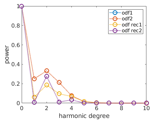
This become clearer when looking at the harmonic coefficients of the reconstructed ODFs. We observe that without ghost correction the recovered odd order harmonic coefficients are much smaller than the original ones.
close all
plotFourier(odf1,'linewidth',2,'bandwidth',10)
hold on
plotFourier(odf2,'linewidth',2)
plotFourier(odf_rec1,'linewidth',2)
plotFourier(odf_rec2,'linewidth',2)
hold off
legend('odf1','odf2','odf rec1','odf rec2')
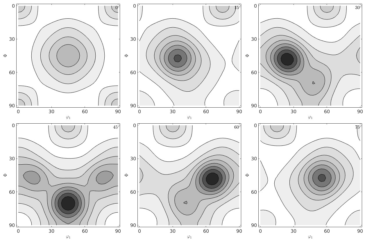
Historically, this effect was is tightly connected with the so-called SantaFe sample ODF.
odf = SantaFe;
plot(odf,'contourf')
mtexColorMap white2black
Let's simulate some diffraction pole figures
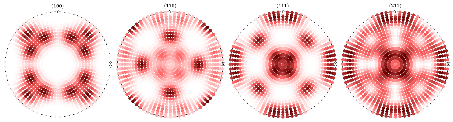
% crystal directions
h = Miller({1,0,0},{1,1,0},{1,1,1},{2,1,1},odf.CS);

% simulate pole figures
pf = calcPoleFigure(SantaFe,h,'antipodal');

% plot them
plot(pf,'MarkerSize',5)
mtexColorMap LaboTeX
and compute two ODFs from them
% one with Ghost Correction
rec = calcODF(pf,'silent')

% one without Ghost Correction
rec2 = calcODF(pf,'NoGhostCorrection','silent')
rec = ODF
  crystal symmetry : m-3m
  specimen symmetry: 222

  Uniform portion:
    weight: 0.73051

  Radially symmetric portion:
    kernel: de la Vallee Poussin, halfwidth 10°
    center: 1219 orientations, resolution: 5°
    weight: 0.26949


rec2 = ODF
  crystal symmetry : m-3m
  specimen symmetry: 222

  Radially symmetric portion:
    kernel: de la Vallee Poussin, halfwidth 10°
    center: 1231 orientations, resolution: 5°
    weight: 1
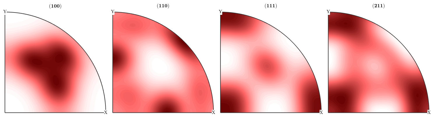
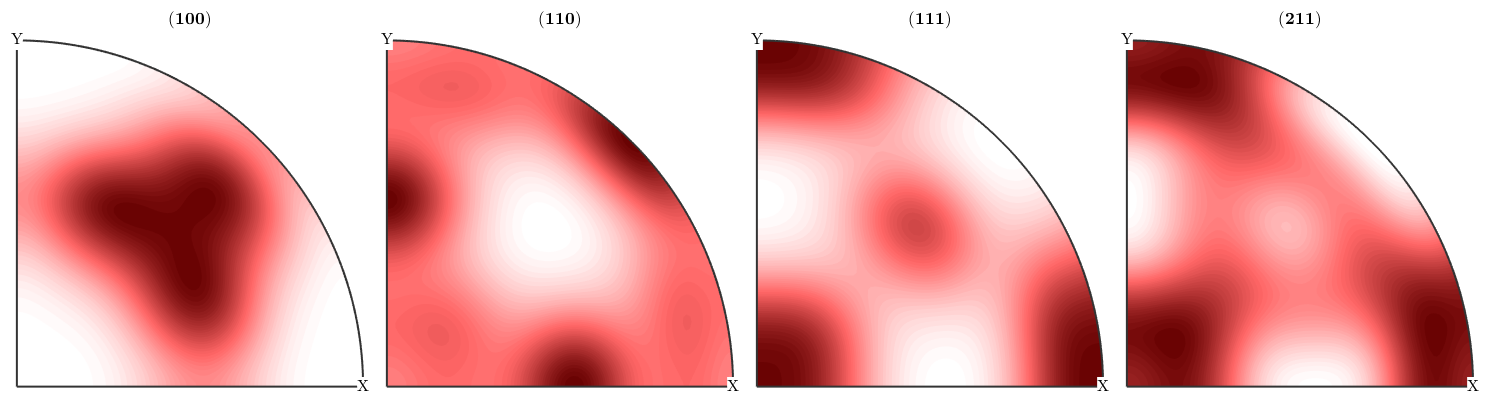
For both reconstruction recalculated pole figures look the same as the initial pole figures
figure(1)
plotPDF(rec,pf.h,'antipodal')
mtexColorMap LaboTeX
figure(2)
plotPDF(rec2,pf.h,'antipodal')
mtexColorMap LaboTeX
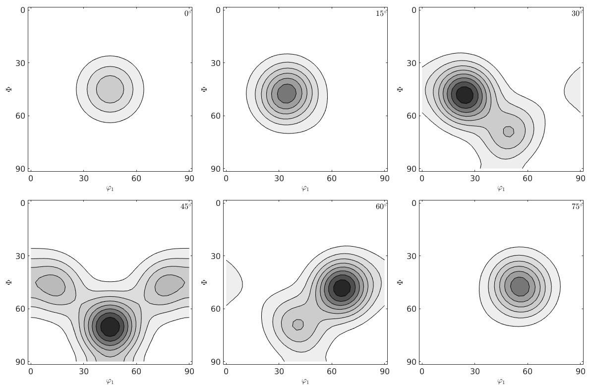
However if we look at the ODF we see big differences. The so-called ghosts.
figure(1)
plot(rec,'gray','contourf')
mtexColorMap white2black
progress: 100%
figure(2)
plot(rec2,'gray','contourf')
mtexColorMap white2black
progress: 100%
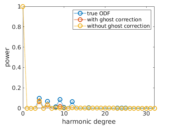
Again we can see the source of the problem in the harmonic coefficients.
close all;
% the harmonic coefficients of the sample ODF
plotFourier(SantaFe,'bandwidth',32,'linewidth',2,'MarkerSize',10)

% keep plot for adding the next plots
hold all

% the harmonic coefficients of the reconstruction with ghost correction:
plotFourier(rec,'bandwidth',32,'linewidth',2,'MarkerSize',10)

% the harmonic coefficients of the reconstruction without ghost correction:
plotFourier(rec2,'bandwidth',32,'linewidth',2,'MarkerSize',10)

legend({'true ODF','with ghost correction','without ghost correction'})
% next plot command overwrites plot
hold off
| DocHelp 0.1 beta |