Simulating Pole Figure data
Simulate arbitrary pole figure data
| On this page ... |
| Introduction |
| Simulate Pole Figure Data |
| ODF Estimation from Pole Figure Data |
| Exploration of the relationship between estimation error and number of single orientations |
Introduction
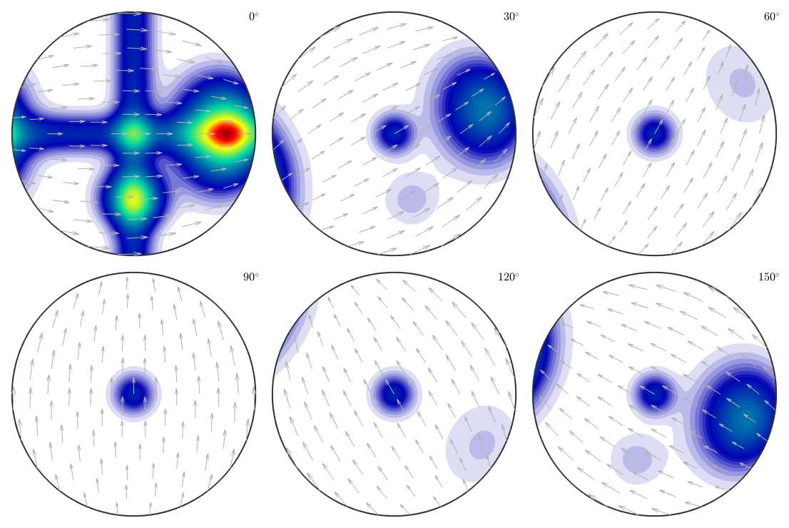
MTEX allows to simulate an arbitrary number of pole figure data from any ODF. This is quite helpful if you want to analyze the pole figure to ODF estimation routine. Let us start with a model ODF given as the superposition of 6 components.
cs = crystalSymmetry('orthorhombic');
mod1 = orientation.byAxisAngle(xvector,45*degree,cs);
mod2 = orientation.byAxisAngle(yvector,65*degree,cs);
model_odf = 0.5*uniformODF(cs) + ...
  0.05*fibreODF(Miller(1,0,0,cs),xvector,'halfwidth',10*degree) + ...
  0.05*fibreODF(Miller(0,1,0,cs),yvector,'halfwidth',10*degree) + ...
  0.05*fibreODF(Miller(0,0,1,cs),zvector,'halfwidth',10*degree) + ...
  0.05*unimodalODF(mod1,'halfwidth',15*degree) + ...
  0.3*unimodalODF(mod2,'halfwidth',25*degree);
plot(model_odf,'sections',6,'silent','sigma')
Simulate Pole Figure Data
In order to simulate pole figure data, the following parameters have to be specified
- an arbitrary ODF
- a list of Miller indece
- a grid of specimen directions
- superposition coefficients (optional)
- the magnitude of error (optional)
The list of Miller indece
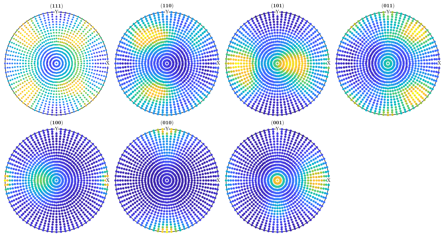
h = [Miller(1,1,1,cs),Miller(1,1,0,cs),Miller(1,0,1,cs),Miller(0,1,1,cs),...
  Miller(1,0,0,cs),Miller(0,1,0,cs),Miller(0,0,1,cs)];
The grid of specimen directions
r = regularS2Grid('resolution',5*degree);Now the pole figures can be simulated using the command calcPoleFigure.
pf = calcPoleFigure(model_odf,h,r)
pf = PoleFigure
  crystal symmetry : mmm
  specimen symmetry: 1

  h = (111), r = 72 x 37 points
  h = (110), r = 72 x 37 points
  h = (101), r = 72 x 37 points
  h = (011), r = 72 x 37 points
  h = (100), r = 72 x 37 points
  h = (010), r = 72 x 37 points
  h = (001), r = 72 x 37 points
Add some noise to the data. Here we assume that the mean intensity is 1000.
pf = noisepf(pf,1000);
Plot the simulated pole figures.
plot(pf)
ODF Estimation from Pole Figure Data
From these simulated pole figures we can now estimate an ODF,
odf = calcODF(pf)
odf = ODF
  crystal symmetry : mmm
  specimen symmetry: 1

  Uniform portion:
    weight: 0.45625

  Radially symmetric portion:
    kernel: de la Vallee Poussin, halfwidth 10°
    center: 29750 orientations, resolution: 5°
    weight: 0.54375
which can be plotted,
plot(odf,'sections',6,'silent','sigma')
progress: 100%
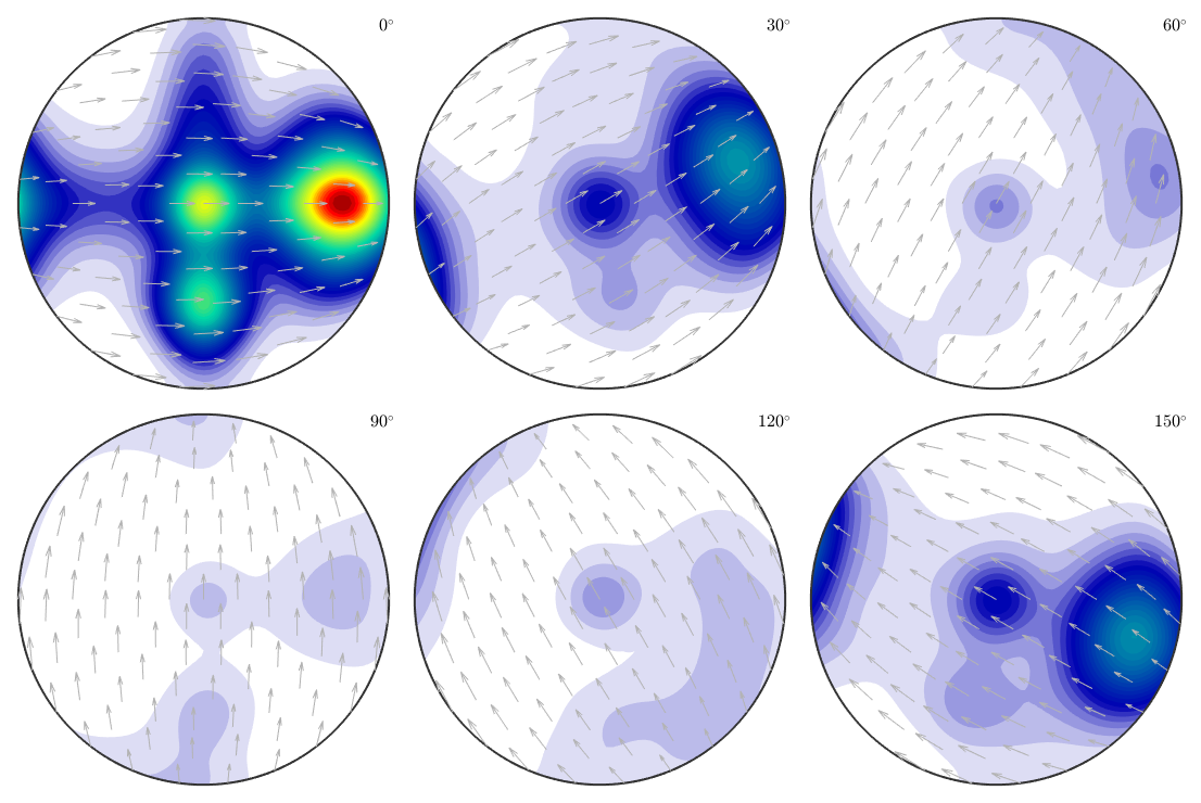
and compared to the original model ODF.
calcError(odf,model_odf,'resolution',5*degree)progress: 100%
ans =
0.0954
Exploration of the relationship between estimation error and number of single orientations
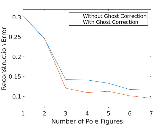
For a more systematic analysis of the estimation error, we vary the number of pole figures used for ODF estimation from 1 to 7 and calculate for any number of pole figures the approximation error. Furthermore, we also apply ghost correction and compare the approximation error to the previous reconstructions.
e = [];
for i = 1:pf.numPF

  odf = calcODF(pf({1:i}),'silent','NoGhostCorrection');
  e(i,1) = calcError(odf,model_odf,'resolution',2.5*degree);
  odf = calcODF(pf({1:i}),'silent');
  e(i,2) = calcError(odf,model_odf,'resolution',2.5*degree);

end
progress: 99%
progress: 99%
progress: 99%
progress: 99%
progress: 99%
progress: 99%
progress: 99%
progress: 99%
progress: 99%
progress: 99%
progress: 99%
progress: 99%
progress: 99%
progress: 99%
Plot the error in dependency of the number of single orientations.
close all;
plot(1:pf.numPF,e)
ylim([0.07 0.32])
xlabel('Number of Pole Figures');
ylabel('Reconstruction Error');
legend({'Without Ghost Correction','With Ghost Correction'});
| DocHelp 0.1 beta |