First Steps
Get in touch with PoleFigure Data in MTEX.
| On this page ... |
| Import of Pole Figures |
| Plotting Pole Figure Data |
| Modify Pole Figure Data |
| Calculate an ODF from Pole Figure Data |
| Simulate Pole Figure Data |
Import of Pole Figures
The most comfortable way to import pole figure data into MTEX is to use the import wizard, which can be started by the command
import_wizard
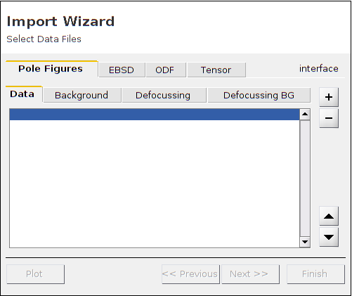
If the data are in a format supported by MTEX the import wizard generates a script which imports the data. More information about the import wizard and a list of supported file formats can be found here. A typical script generated by the import wizard looks as follows:
% specify scrystal and specimen symmetry
cs = crystalSymmetry('32',[1.4,1.4,1.5]);

% specify file names
fname = {...
  fullfile(mtexDataPath,'PoleFigure','dubna','Q(10-10)_amp.cnv'),...
  fullfile(mtexDataPath,'PoleFigure','dubna','Q(10-11)(01-11)_amp.cnv'),...
  fullfile(mtexDataPath,'PoleFigure','dubna','Q(11-22)_amp.cnv')};

% specify crystal directions
h = {Miller(1,0,-1,0,cs),[Miller(0,1,-1,1,cs),Miller(1,0,-1,1,cs)],Miller(1,1,-2,2,cs)};

% specify structure coefficients
c = {1,[0.52 ,1.23],1};

% import pole figure data
pf = PoleFigure.load(fname,h,cs,'superposition',c)

% After running the script the variable *pf* is created which contains all
% information about the pole figure data.
pf = PoleFigure
  crystal symmetry : 321, X||a*, Y||b, Z||c*
  specimen symmetry: 1

  h = (10-10), r = 72 x 19 points
  h = (01-11)(10-11), r = 72 x 19 points
  h = (11-22), r = 72 x 19 points
Plotting Pole Figure Data
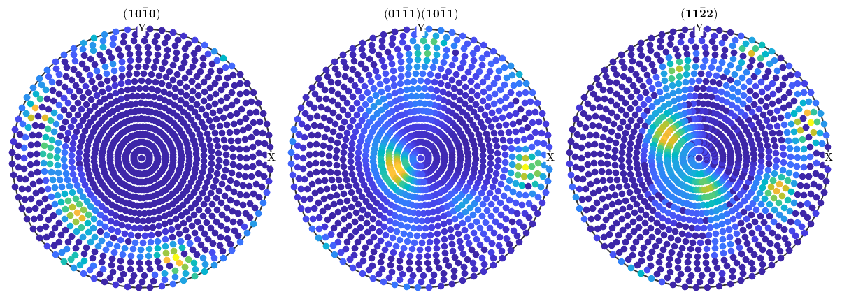
Pole figures are plotted using the plot command. It plots a single colored dot for any data point contained in the pole figure. There are many options to specify the way pole figures are plotted in MTEX. Have a look at the plotting section for more information.
plot(pf)
Modify Pole Figure Data
MTEX offers a lot of operations to analyze and manipulate pole figure data, e.g.
- rotating pole figures
- scaling pole figures
- find outliers
- remove specific measurements
- superpose pole figures
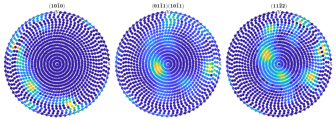
An exhaustive introduction how to modify pole figure data can be found here As an example if one wants to set all negative intensities to zero one can issue the command
pf(pf.intensities<0) = 0;
plot(pf)
Calculate an ODF from Pole Figure Data
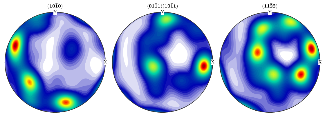
Calculating an ODF from pole figure data can be done using the command calcODF. A precise description of the underlying algorithm as well as of the options can be found here
odf = calcODF(pf,'zero_range','silent')
plotPDF(odf,h,'antipodal','superposition',c)
odf = ODF
  crystal symmetry : 321, X||a*, Y||b, Z||c*
  specimen symmetry: 1

  Radially symmetric portion:
    kernel: de la Vallee Poussin, halfwidth 10°
    center: 19831 orientations, resolution: 5°
    weight: 1
Simulate Pole Figure Data
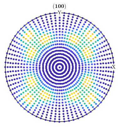
Simulating pole figure data from a given ODF has been proved to be useful to analyze the stability of the ODF estimation process. There is an example demonstrating how to determine the number of pole figures to estimate the ODF up to a given error. The MTEX command to simulate pole figure is calcPoleFigure, e.g.
pf = calcPoleFigure(SantaFe,Miller(1,0,0,crystalSymmetry('m-3m')),regularS2Grid)
plot(pf)
pf = PoleFigure crystal symmetry : m-3m specimen symmetry: 222 h = (100), r = 72 x 37 points
| DocHelp 0.1 beta |