Authors: Vivian Tong. EBSD data from "Void-Microstructure Correlation in Thin Film Copper Power Semiconductor Metallization using MTEX", Matthias Grabner, Master's Thesis, Graz University of Technology, 2023. Contact: vivian.tong@extern.tu-freiberg.de
Thin film copper metallization develops voids as it ages. A void is a hole, so EBSD has nothing to index there and only the electron image sees it, while the grain boundaries the void may or may not sit on are visible only to EBSD. Neither dataset can answer where the voids are, and both together can - once they overlay pixel for pixel.
This page aligns the two with TrueEBSD and then asks the two questions that alignment makes answerable:
- do the voids sit on grain boundaries and triple junctions, or anywhere?
- are some boundary types more resistant to voiding than others?
The alignment half of the workflow is explained step by step in TrueEBSD on a WC-Co composite — read that one first if you are new to TrueEBSD. This page keeps the alignment brief and spends its time on the voids.
It needs the TrueEBSD toolbox, which is not part of MTEX and is distributed separately under Apache-2.0: https://github.com/vtvivian/mtex-trueebsd
addpath(genpath('<path to mtex-trueEbsd>'))Use the mtex7-compat branch with MTEX 7. Beyond MTEX it requires MATLAB R2024a or newer and the Image Processing, Curve Fitting, and Statistics and Machine Learning toolboxes. Runtime is minutes, not seconds.
Data Import
The data set is a single Oxford Instruments .h5oina file holding both the EBSD map and the SEM images of the same area. It is 164 MB and is not shipped with MTEX, so it is downloaded on first use from Zenodo: zenodo.org/records/16902083.
fName = fullfile(mtexDataPath,'EBSD','copper29.h5oina');

if ~isfile(fName)
  websave(fName,'https://zenodo.org/records/16902083/files/copper29.h5oina');
end
Everything in this file came out of one acquisition, so the map and the images are stored the same way round and TrueEBSD works that out for itself. The frames page is the case where they are not.
The convention set here only decides which way up the figures come out. It has no effect on the correction.
plottingConvention.default('y↓→x')

ebsd = EBSD.load(fName)
ans = plottingConvention (y↓→x)
════════════════════════════════════════════════════════════════════════════════
HDF5 CONFIGURATION LOADED
├── Manufacturer : Oxford
├── Info : A map may be stored twice - as recorded by the detector under
'EBSD' and as cleaned up by the vendor software under 'Data Processing'. Both
are offered as data sets, the cleaned up one first.
════════════════════════════════════════════════════════════════════════════════
ebsd = EBSDsquare (Y1↓→X1)
Phase Orientations Mineral Color Symmetry Crystal reference frame
0 52244 (9.3%) notIndexed none
1 511713 (91%) Copper LightSkyBlue m-3m
Properties: BandContrast, BandSlope, Bands, BeamPositionX, BeamPositionY, DetectorDistance, Error, MeanAngularDeviation, PatternCenterX, PatternCenterY, PatternQuality, oldId
Scan unit : um
X x Y x Z : [0 → 103] x [0 → 55] x [0 → 0]
Normal vector: (0,0,1)
Square grid :547 x 1031
dataSet: /1/EBSD
dataSets: /1/EBSDThe images that ship inside the .h5oina container come back in ebsd.opt.electron_image, one field per detector, plus a Header that states their pixel size. This file holds 24 of them; three are used here.
- Band contrast is the image belonging to the EBSD map. The
.h5oinaloader names the map properties after the HDF5 data sets, so it arrives asebsd.BandContrastrather than under the short namebcthe.ctfloader uses.
-
LowerCentre19,LowerLeft19andLowerRight19are the three FSD detectors mounted at the bottom of the EBSD camera, with the camera retracted by 40 mm relative to the EBSD map acquisition position. They are stacked into one colour image.
-
ABSinner_0degis a greyscale image from the annular backscatter (ABS) detector at 10 kV and 0 degrees sample tilt.
semImgs = ebsd.opt.electron_imagesemImgs =
struct with fields:
LowerCentre19: [1280×2048 double]
LowerCentre20: [1280×2048 double]
LowerCentre21: [1280×2048 double]
LowerLeft19: [1280×2048 double]
LowerLeft20: [1280×2048 double]
LowerLeft21: [1280×2048 double]
LowerRight19: [1280×2048 double]
LowerRight20: [1280×2048 double]
LowerRight21: [1280×2048 double]
UpperLeft19: [1280×2048 double]
UpperLeft20: [1280×2048 double]
UpperLeft21: [1280×2048 double]
UpperRight19: [1280×2048 double]
UpperRight20: [1280×2048 double]
UpperRight21: [1280×2048 double]
ABSinner_0deg: [1280×2048 double]
CBS_0deg_immersion: [1280×2048 double]
CBS_0deg_immersion_20kV: [1280×2048 double]
CBSab_0deg: [1280×2048 double]
ETD_0deg: [1280×2048 double]
ETD_70deg: [1280×2048 double]
T1_0deg: [1280×2048 double]
T1_0deg_immersion: [1280×2048 double]
T1_70deg: [1280×2048 double]
Header: [1×1 struct]The backscatter image is filtered two ways, because the two things we need from it respond to opposite treatments. bse1a is raised to a high power, which pulls the mid greys apart and brings up grain boundary contrast, and is what the registration needs. bse1b gets a moving median, which preserves the edges of the voids and is what the analysis needs.
fsd1B = rescale(im2double(cat(3,semImgs.LowerCentre19, ...
  semImgs.LowerLeft19, ...
  semImgs.LowerRight19)));
bse1  = rescale(im2double(semImgs.ABSinner_0deg));

fsd1a = imboxfilt(fsd1B,5);
bse1a = imboxfilt(bse1.^10,5);
bse1b = medfilt2(bse1,[3 3],'symmetric');
Build the sequence
TrueEBSD steps from the EBSD map to the reference image one pair at a time, correcting one kind of distortion at each step. The sequence runs from the most distorted to the one you trust, and each entry names the distortion between itself and the next one.
Images 3 and 4 are the same backscatter image filtered two different ways, so nothing physically separates them and both are marked 'true'. Image 4 is deliberately filtered to show voids rather than grain boundaries, which leaves it with almost no boundary contrast to match on — hence 'highContrast',0, which tells TrueEBSD to borrow the previous image's contrast for that step instead.
'name' is what each image is called once it is attached to the map at the end, so everything below reads ebsd.bse1b rather than juggling separate arrays.
dxyImg = double(semImgs.Header.XStep);

imgList = createArray(4,1,'distortedImg');
imgList(1) = distortedImg('BandContrast','shift-drift', ebsd, 'name','bcImg', ...
  'highContrast',1, 'edgePadWidth',3);
imgList(2) = distortedImg(fsd1a,'tilt', 'dxy', dxyImg, 'name','fsd1a', 'highContrast',1, 'edgePadWidth',3);
imgList(3) = distortedImg(bse1a,'true', 'dxy', dxyImg, 'name','bse1a', 'highContrast',1, 'edgePadWidth',3);
imgList(4) = distortedImg(bse1b,'true', 'dxy', dxyImg, 'name','bse1b', 'highContrast',0, 'edgePadWidth',1);

job = trueEbsd(imgList)
job = trueEbsd (as imported)
image distortion shift residual
1 547 x 1031 shift-drift - -
2 1280 x 2048 x 3 tilt - -
3 1280 x 2048 true - -
4 1280 x 2048 true - -Plot the as-imported sequence to check that the maps cover similar regions of the sample.
plot(imgList,'TrueEBSD starting image sequence')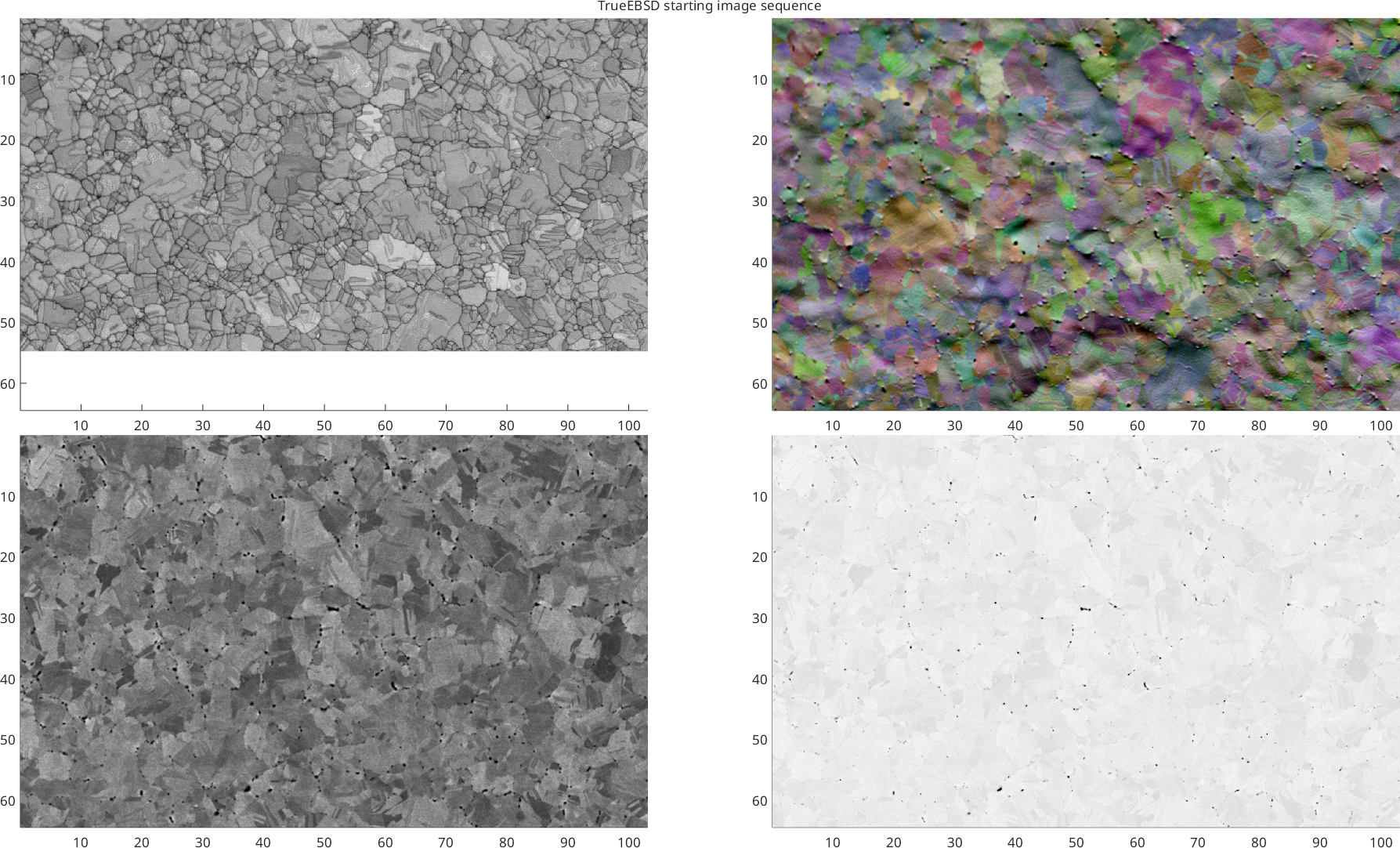
Align the sequence
Three steps, the same as in the WC-Co example: put everything on one pixel grid, measure the distortion between each pair by matching small boxes across them, then apply the accumulated shifts.
pixSzIn = 0; % target pixel length in microns, or 0 for the smallest present
job.pixelSizeMatch(pixSzIn);
using default pixel size of 0.050355 um, minimum from imgListThese are the pictures that will actually be matched: edge transforms where xcfImg is 'edge', grey values where it is 'img'. A band contrast map and a backscatter image have nothing in common as grey values, but their grain boundaries fall in the same places.
plot(job.resizedList,'TrueEBSD image sequence for cross-correlation','xcf')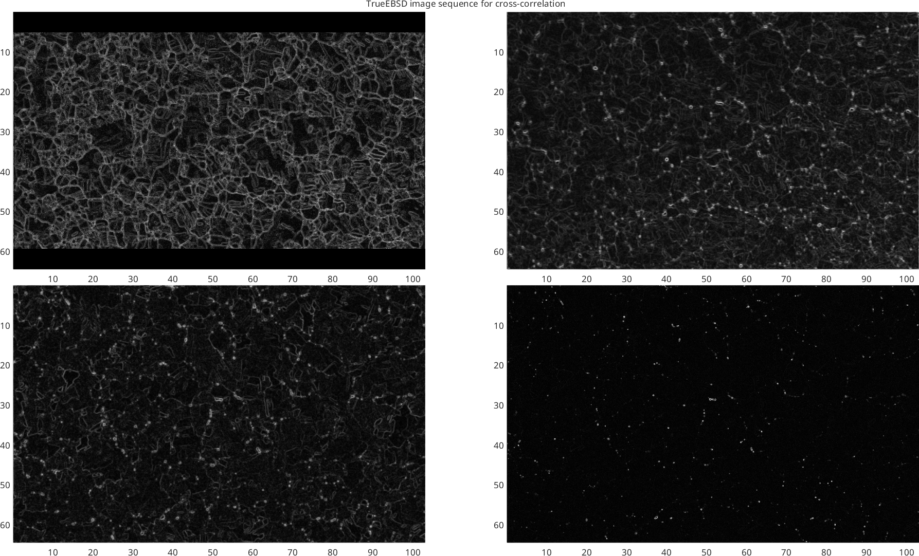
'fitErr' re-measures the shifts after each correction and reports what is left over. Around a pixel or less means it worked. Those residuals are kept in job.fitError, and they matter later on this page: they set how large a void has to be before its position can be trusted.
job.calcDistortion('fitErr')fitting the distortion across 4 maps, 3 hops
hop distortion model ROI shift residual
2→1 shift-drift poly11 512 px 67.79 px
linearinterp 512 px 0.72 px
after fitting 0.47 px
Warning: Iteration limit reached.
3→2 tilt projective 512 px 126.77 px
poly11 512 px 5.25 px
poly22 512 px 1.40 px
after fitting 1.23 px
4→3 true not correlated - 0.00 px
not fitted 0.90 px
ans = trueEbsd (shifts calculated)
image distortion shift residual
1 1280 x 2048 shift-drift 2.1 px 0.47 px
2 1280 x 2048 x 3 tilt 1.9 px 1.2 px
3 1280 x 2048 true 0 px 0.9 px
4 1280 x 2048 true - -
common grid: 1280 x 2048 at 0.05 µmjob.undistort
plot(job.undistortedList,'TrueEBSD image sequence after alignment')ans = trueEbsd (undistorted)
image distortion shift residual
1 1280 x 2048 shift-drift 2.1 px 0.47 px
2 1280 x 2048 x 3 tilt 1.9 px 1.2 px
3 1280 x 2048 true 0 px 0.9 px
4 1280 x 2048 true - -
common grid: 1280 x 2048 at 0.05 µm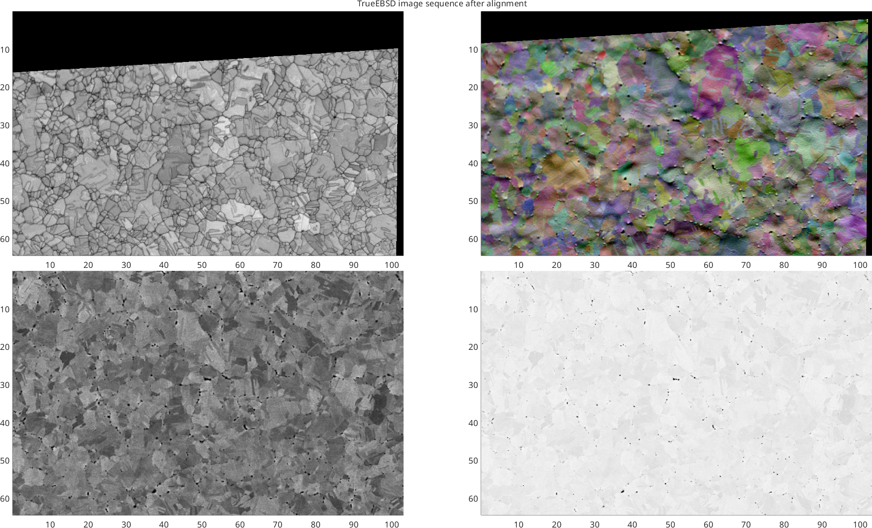
Use the result
Every image is now attached to the EBSD map as a per-pixel property, under the 'name' given earlier. So ebsd.bse1b is just another map property, and plot(ebsd,ebsd.bse1b) works like any other plot — no conversion, and it stays with the map through cropping, gridding and indexing. That is what the whole voids analysis below rests on.
Plotting them back onto the map is also the quickest check that nothing came out the wrong way round.
ebsdOut = job.undistortedList(1).ebsd;

figure
nextAxis
plot(ebsdOut('indexed'), ebsdOut('indexed').orientations, 'coordinates','on')
title('Undistorted MTEX EBSD map (Copper IPF out of screen)','Color','k')

for n = 1:numel(job.undistortedList)

  % a colour image keeps its channels as a property, and plotting values
  % onto a map needs one per pixel
  im = ebsdOut.(job.undistortedList(n).name);
  if size(im,3) > 1, im = mean(im,3); end

  nextAxis
  plot(ebsdOut, im, 'coordinates','on')
  mtexColorMap gray
  title(['Undistorted ' job.undistortedList(n).name],'Color','k')
end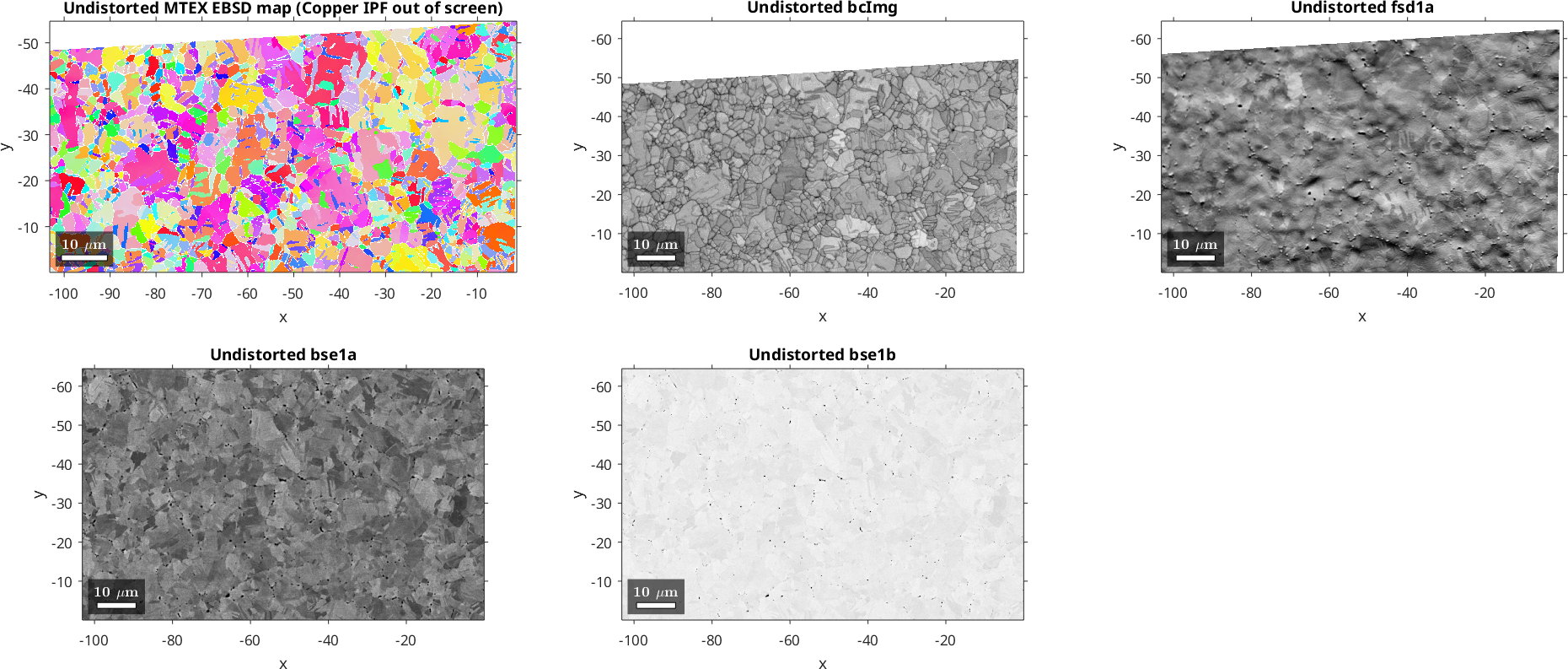
Turn the voids into a phase
That is the end of the distortion correction. Everything below is ordinary MTEX on an EBSD map that now carries its images pixel for pixel.
Correcting the distortion moves the EBSD map within its grid, so it comes back with a border of points it never covered. trim cuts a gridded map down to the smallest rectangle holding all of its indexed data. The images ride along, because they are properties of the map now — there is no second array to keep in step, and no question of whether it is indexed the same way round.
That rectangle is not covered completely: the correction rotates and shears the map a little, so its own coverage is a quadrilateral and the corners of the rectangle stay not indexed, with the aligned band contrast NaN there. The backscatter image covers all of it, being the reference.
ebsd = trim(job.undistortedList(1).ebsd)ebsd = EBSDsquare (Y1↓→X1)
Phase Orientations Mineral Color Symmetry Crystal reference frame
0 326627 (15%) notIndexed none
1 1867093 (85%) Copper LightSkyBlue m-3m
Properties: BandContrast, BandSlope, Bands, BeamPositionX, BeamPositionY, DetectorDistance, Error, MeanAngularDeviation, PatternCenterX, PatternCenterY, PatternQuality, oldId, bcImg, fsd1a, bse1a, bse1b
Scan unit : um
X x Y x Z : [-103 → -1] x [-55 → 0] x [0 → 0]
Normal vector: (0,0,1)
Square grid :1086 x 2020A void is a hole, so the aligned backscatter image is the only evidence of where it is. Thresholding that image gives a mask, and the mask becomes a phase of its own — which is what makes the voids available to calcGrains, grains.boundary and every other MTEX tool below.
The natural phase for a hole is a named not indexed one. A void carries no orientation, and notIndexed takes a name and a colour, so the voids stay selectable as ebsd('voids') and stay out of ebsd('indexed') without being given a fake symmetry and a fake identity orientation. Adding a phase means appending it to ebsd.CSList and ebsd.phaseMap; after that the pixels are labelled by name.
The threshold is asked of the uncovered corners as well, where the backscatter image is defined but the EBSD map never reached. A dark pixel there is missing data rather than a void, so the mask is restricted to the map's own coverage — which is exactly where the aligned band contrast is not NaN. Without that restriction 7% more pixels are called voids, in a region where no boundary was measured to attribute them to.
voidThreshold = 0.8;                % backscatter level below which a pixel is a void
voidColor     = str2rgb('DarkBlue');

ebsd.CSList(end+1)   = notIndexed('voids',voidColor);
ebsd.phaseMap(end+1) = max(ebsd.phaseMap) + 1;

isVoid = ebsd.bse1b < voidThreshold & ~isnan(ebsd.bcImg);

ebsd(isVoid) = 'voids'
ebsd = EBSDsquare (Y1↓→X1)
Phase Orientations Mineral Color Symmetry Crystal reference frame
0 322926 (15%) notIndexed none
1 1856205 (85%) Copper LightSkyBlue m-3m
2 14589 (0.67%) voids DarkBlue
Properties: BandContrast, BandSlope, Bands, BeamPositionX, BeamPositionY, DetectorDistance, Error, MeanAngularDeviation, PatternCenterX, PatternCenterY, PatternQuality, oldId, bcImg, fsd1a, bse1a, bse1b
Scan unit : um
X x Y x Z : [-103 → -1] x [-55 → 0] x [0 → 0]
Normal vector: (0,0,1)
Square grid :1086 x 2020The voids as objects
The mask says which pixels are dark. To speak of a void we need the pixels grouped into connected objects, which is what calcGrains does for any phase, indexed or not.
Two of its parameters do the work here. 'minPixel' is the smallest number of pixels that still counts as a grain; pixels of anything smaller are marked not indexed, which is how the isolated speckles of the threshold are separated from the real voids. 'alpha' is the radius, in pixels, of the smallest not indexed region that is not absorbed into the surrounding grains — it defaults to 3.1, and 'alpha',0 keeps every not indexed region, so the voids survive as objects of their own. The next section uses the opposite setting.
[voidGrains,ebsd] = calcGrains(ebsd,'angle',10*degree,'alpha',0,'minPixel',5);

voids = voidGrains('voids')

% which void a pixel belongs to - the second reconstruction overwrites this
voidId = ebsd.grainId;

fprintf('%d voids, %d of the %d masked pixels (%.0f %%) belong to one\n', ...
  length(voids), sum(voids.numPixel), nnz(isVoid), ...
  100*sum(voids.numPixel)/nnz(isVoid));
fprintf('void diameter: median %.1f pixels, 90th percentile %.1f pixels\n', ...
  median(voids.equivalentRadius)*2/ebsd.dPos, ...
  prctile(voids.equivalentRadius,90)*2/ebsd.dPos);

figure
histogram(voids.area,50);
xlabel('void area ({\mu}m^2)'); ylabel('number of voids');
voids = grain2d (Y1↓→X1)
Phase Grains Pixels Mineral Symmetry Color
2 531 13524 voids DarkBlue
boundary segments: 11840 (596 µm)
inner boundary segments: 0 (0 µm)
triple points: 1502
Properties: meanRotation, GOS
531 voids, 13524 of the 14589 masked pixels (93 %) belong to one
void diameter: median 4.5 pixels, 90th percentile 8.6 pixels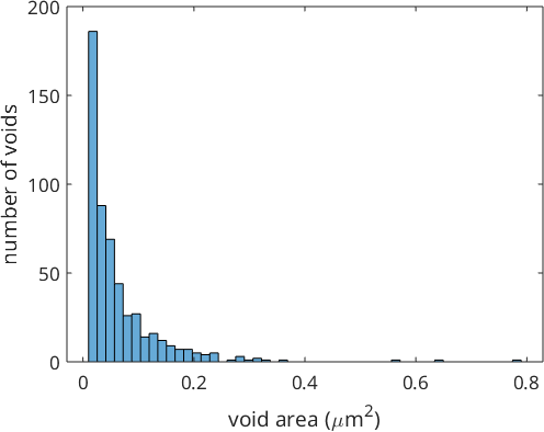
Close the boundary network over the voids
Now the same reconstruction with the opposite 'alpha'. The voids are a few pixels across, so 'alpha',6 swallows all but the largest of them and they are absorbed into the copper grains around them. Where two grains surround the same void they meet inside it, and the boundary between them runs straight through the hole instead of stopping at its edge.
That is the whole trick of this page. A void does not have to be matched to a boundary by distance or by any threshold: the reconstruction closes the network over it, and which grains meet inside a void says where the void sits. Anything from 'alpha',6 to 'alpha',20 gives the same answer here, since the voids are far smaller than the grains.
[grains,ebsd] = calcGrains(ebsd,'angle',10*degree,'alpha',6,'minPixel',5)

cu  = grains('Copper');
gBs = grains.boundary('Copper','Copper');   % naming both phases drops the map border

% which copper grain a pixel belongs to now, voids included
grainOfPixel = ebsd.grainId;
isCu = ismember(grainOfPixel,cu.id);
grains = grain2d (Y1↓→X1)
Phase Grains Pixels Mineral Symmetry Color
1 2379 1854231 Copper m-3m LightSkyBlue
2 1 168 voids DarkBlue
boundary segments: 134622 (7736 µm)
inner boundary segments: 5 (0.24 µm)
triple points: 4143
Properties: meanRotation, GOS
ebsd = EBSDsquare (Y1↓→X1)
Phase Orientations Mineral Color Symmetry Crystal reference frame
0 183982 (8.4%) notIndexed none
1 2009550 (92%) Copper LightSkyBlue m-3m
2 188 (0.0086%) voids DarkBlue
Properties: BandContrast, BandSlope, Bands, BeamPositionX, BeamPositionY, DetectorDistance, Error, MeanAngularDeviation, PatternCenterX, PatternCenterY, PatternQuality, oldId, bcImg, fsd1a, bse1a, bse1b, grainId
Scan unit : um
X x Y x Z : [-103 → -1] x [-55 → 0] x [0 → 0]
Normal vector: (0,0,1)
Square grid :1086 x 2020The voids are still a phase of the map — calcGrains assigned them to grains, it did not relabel the pixels — so they can be drawn straight onto the band contrast in their own phase colour.
figure; newMtexFigure('layout',[2,1]);
nextAxis
plot(ebsd,ebsd.BandContrast,'micronbar','off');
mtexColorMap gray; hold on
plot(ebsd('voids'),'faceColor',voidColor);
mtexTitle('Band Contrast and Voids');
nextAxis
plot(ebsd('Copper'),ebsd('Copper').orientations,'FaceAlpha',0.5,'micronbar','on'); hold on
plot(gBs,'linewidth',1,'linecolor','g');
plot(ebsd('voids'),'faceColor',voidColor);
mtexTitle('Copper Orientations (IPF out of screen), Grain Boundaries and Voids');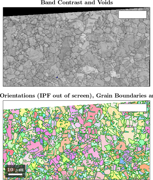
Where does each void sit?
Every pixel now knows two things: which void it belongs to, and which copper grain the closed network gives it. Counting the distinct grains behind one void answers the first question of this page:
- one grain — the void is inside a grain
- two grains — it sits on the boundary between them
- three or more — it sits on a triple junction
inVoid  = ismember(voidId,voids.id) & isCu;

% every (void, grain) pair that occurs, and how many grains each void has
pairs      = unique([voidId(inVoid) grainOfPixel(inVoid)],'rows');
[g,vId]    = findgroups(pairs(:,1));
nGrains    = accumarray(g,1);

fprintf('%d voids: %d inside a grain, %d on a boundary, %d at a junction\n', ...
  numel(vId), nnz(nGrains==1), nnz(nGrains==2), nnz(nGrains>=3));
fprintf('%.0f %% of the voids sit on a boundary or a junction\n', ...
  100*mean(nGrains>=2));
531 voids: 250 inside a grain, 188 on a boundary, 93 at a junction
53 % of the voids sit on a boundary or a junctionHalf of them do — which means nothing until we know the rate a void of the same size reaches by chance. The grains here are only a few tens of pixels across, so a patch dropped anywhere has a fair chance of straddling a boundary, and the honest control is to drop each void shape at random positions and count grains under it the same way.
sz = size(ebsd);
grainMap = reshape(grainOfPixel,sz);
grainMap(~isCu) = 0;                     % 0 wherever there is no copper grain
voidMap = reshape(voidId,sz);

rng(0)
nRandom = zeros(numel(vId),10);

for k = 1:numel(vId)

  % the shape of this void, as offsets from its own top left corner
  [r,c] = find(voidMap == vId(k));
  r = r - min(r) + 1; c = c - min(c) + 1;

  for rep = 1:10
    idx = sub2ind(sz, r + randi(sz(1)-max(r)), c + randi(sz(2)-max(c)));
    % count only the placements that land entirely on copper
    if all(grainMap(idx) > 0), nRandom(k,rep) = numel(unique(grainMap(idx))); end
  end
end

nRandom = nRandom(nRandom > 0);

fprintf('at random: %.0f %% on a boundary or junction, %.0f %% at a junction\n', ...
  100*mean(nRandom>=2), 100*mean(nRandom>=3));
fprintf('measured : %.0f %% on a boundary or junction, %.0f %% at a junction\n', ...
  100*mean(nGrains>=2), 100*mean(nGrains>=3));
at random: 9 % on a boundary or junction, 0 % at a junction
measured : 53 % on a boundary or junction, 18 % at a junctionHow large does a void have to be?
The answer above is a per void yes/no, so it is only as good as the alignment that put the void where it is. The residual local shift left over after each hop of the correction is the natural measure of that, and 'fitErr' kept it in job.fitError. Summed over the hops that were actually fitted, its 95th percentile is the distance a feature may still be off by.
The 'true' hops are left out of that sum. job.fitError holds a residual for them as well, but nothing was fitted there and nothing separates those pairs — images 3 and 4 are the same backscatter image under two filters, neither of which shifts a pixel.
isFitted = arrayfun(@(d) ~isempty(d.distortionModel{1}), ...
  job.resizedList(1:end-1));

resid95 = arrayfun(@(f) ...
  prctile(hypot(f.xShiftsXcf/f.dx, f.yShiftsXcf/f.dy),95), job.fitError);

for n = 1:numel(resid95)
  fprintf('  hop %d (%-11s) 95th percentile residual %.2f px%s\n', ...
    n, job.resizedList(n).distortionName, resid95(n), ...
    string(repmat(' - not counted',1,~isFitted(n))));
end
fprintf('a feature may be off by up to %.2f pixels\n',sum(resid95(isFitted)));
hop 1 (shift-drift) 95th percentile residual 1.02 px
hop 2 (tilt ) 95th percentile residual 2.63 px
hop 3 (true ) 95th percentile residual 1.30 px - not counted
a feature may be off by up to 3.65 pixelsThat is of the order of the median void, so the smallest voids are the ones whose site is least certain. Restricting the count to the voids that are clearly larger than the residual is therefore the robustness check this analysis needs — and it strengthens the result rather than weakening it.
isBig = ismember(vId,voids.id(voids.numPixel >= 20));

fprintf('%d voids of at least 20 pixels: %.0f %% on a boundary or junction\n', ...
  nnz(isBig), 100*mean(nGrains(isBig)>=2));
218 voids of at least 20 pixels: 79 % on a boundary or junctionWhich boundaries resist voids?
The second question. A void that sits on a plain boundary names the two grains it separates, and the misorientation between them is the character of that boundary. Taking every segment between such a pair marks the boundaries that carry a void, so their misorientation distribution can be compared against the distribution over all boundaries — same quantity, same weighting by segment.
Voids at a junction are left out here. They touch three boundaries at once and cannot single out one of them.
onBoundary = vId(nGrains == 2);
grainPair  = reshape(pairs(ismember(pairs(:,1),onBoundary),2),2,[])';

isVoidBnd = ismember(sort(gBs.grainId,2),sort(grainPair,2),'rows');

fprintf('%d of %d boundary segments (%.1f %%) carry a void\n', ...
  nnz(isVoidBnd), length(gBs), 100*mean(isVoidBnd));

figure; newMtexFigure;
plot(ebsd('Copper'),ebsd('Copper').orientations,'FaceAlpha',0.3); hold on
plot(gBs,'linecolor',str2rgb('gray'));
plot(gBs(isVoidBnd),'linecolor',str2rgb('LightGreen'),'linewidth',3);
plot(ebsd('voids'),'faceColor',voidColor);
mtexTitle('The boundaries that carry a void');
4948 of 128378 boundary segments (3.9 %) carry a void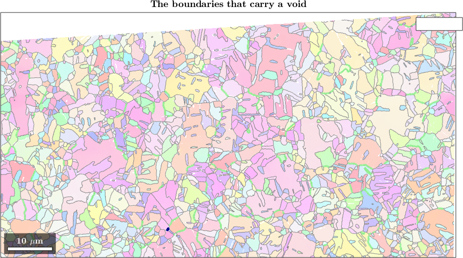
The answer is in the next two plots. The boundaries that carry voids are depleted of 60 degree misorientations about [111] — the sigma-3 twin boundaries of FCC copper — while the material as a whole is full of them. Twins resist void formation.
sigma3 = orientation.byAxisAngle(Miller(1,1,1,cu.CS),60*degree,cu.CS,cu.CS);

fprintf('within 3 degree of the sigma-3 twin: %.0f %% of all boundaries, ', ...
  100*mean(angle(gBs.misorientation,sigma3) < 3*degree));
fprintf('%.0f %% of the void boundaries\n', ...
  100*mean(angle(gBs(isVoidBnd).misorientation,sigma3) < 3*degree));

mdfAll  = calcDensity(gBs.misorientation);
mdfVoid = calcDensity(gBs(isVoidBnd).misorientation);

figure
newMtexFigure('figSize','tiny','outerplotspacing',30);
plotAngleDistribution(mdfAll,'DisplayName','All GBs'); hold on
plotAngleDistribution(mdfVoid,'DisplayName','Void GBs');
plotAngleDistribution(cu.CS,cu.CS,'antipodal','DisplayName','Uniform MDF');
legend('show','Location','northwest');
xlabel('Misorientation angle / degrees');
ylabel('Frequency / mrd');
within 3 degree of the sigma-3 twin: 62 % of all boundaries, 28 % of the void boundaries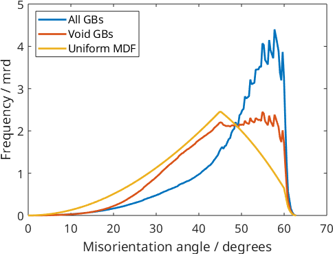
The axis distributions say the same thing in the other coordinate: the [111] pole that dominates all boundaries is much weaker among the ones that carry a void.
figure; newMtexFigure('layout',[1,3],'figSize','large','outerplotspacing',30,'innerplotspacing',50);
nextAxis(1,1); plotAxisDistribution(mdfAll,'colorRange','equal'); mtexTitle('All GBs');
nextAxis(1,2); plotAxisDistribution(mdfVoid,'colorRange','equal'); mtexTitle('Void GBs');
nextAxis(1,3); plotAxisDistribution(cu.CS,cu.CS,'antipodal','colorRange','equal');
mtexTitle('Uniform MDF');
mtexColorbar;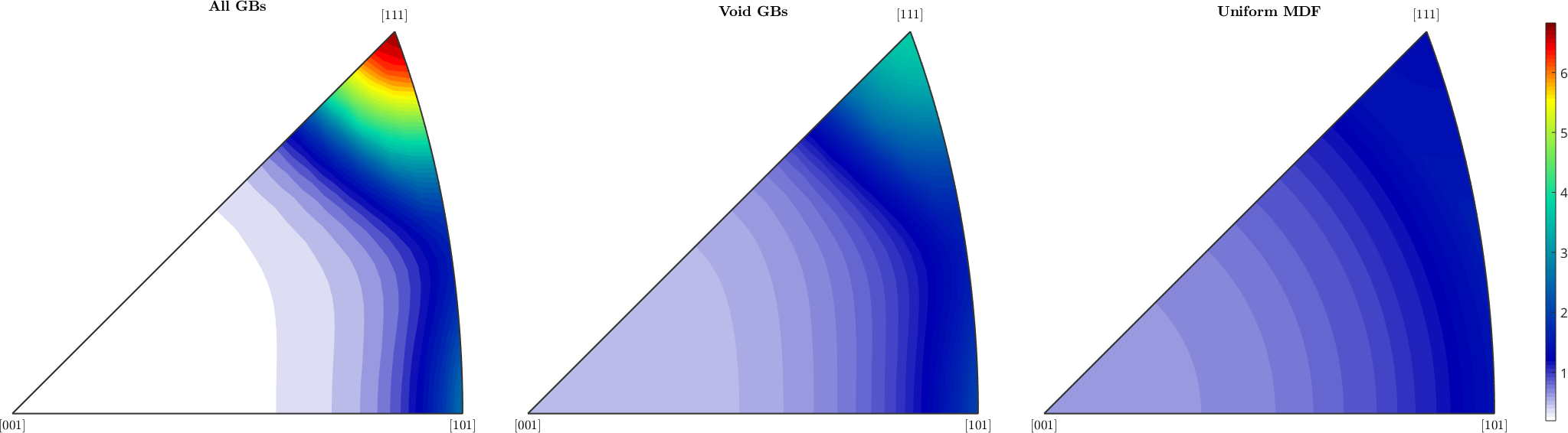
Both answers came out of one EBSD variable. The voids entered it as a threshold on an image property, the boundaries came from the orientations, and nothing below the alignment had to know that the two were ever separate datasets — which is what the distortion correction at the top of this page was for.
Citing this page.
This page is part of the documentation of
MTEX, a free and open
source MATLAB toolbox for analyzing and modeling crystallographic textures.
It was written by The MTEX Developers and is published at
https://mtex-toolbox.github.io/example_copper.html.
If you use MTEX, or reuse text or figures from this page, in your research,
please cite
F. Bachmann, R. Hielscher, H. Schaeben: Texture Analysis with MTEX - Free and Open Source Software Toolbox, Solid State Phenomena 160 (2010), 63-68. 10.4028/www.scientific.net/SSP.160.63
BibTeX
@article{bachmann2010mtex,
  author  = {F. Bachmann and R. Hielscher and H. Schaeben},
  title   = {Texture Analysis with MTEX - Free and Open Source Software Toolbox},
  journal = {Solid State Phenomena},
  volume  = {160},
  pages   = {63-68},
  year    = {2010},
  doi     = {10.4028/www.scientific.net/SSP.160.63},
  url     = {https://doi.org/10.4028/www.scientific.net/SSP.160.63}
}
Other papers describing specific MTEX methods are listed under Publications — please cite the one that best fits your application. The MTEX source code is licensed under the GNU General Public License v2.0; the text and figures of this documentation are licensed under CC BY 4.0, which permits reuse — including by automated systems — provided The MTEX Developers and this page are credited.