MTEX - Analysis of EBSD Data

Analysis of single orientation measurement.

Specify Crystal and Specimen Symmetry

% specify crystal and specimen symmetry
CS = {...
  'Not Indexed',...
  crystalSymmetry('m-3m','mineral','Fe'),... % crystal symmetry phase 1
  crystalSymmetry('m-3m','mineral','Mg')};   % crystal symmetry phase 2

import ebsd data

% file name
fname = fullfile(mtexDataPath,'EBSD','85_829grad_07_09_06.txt');

ebsd = EBSD.load(fname,'CS',CS,...
  'ColumnNames', { 'Phase' 'x' 'y' 'Euler 1' 'Euler 2' 'Euler 3' 'Mad' 'BC'},...
  'Columns', [2 3 4 5 6 7 8 9],...
  'ignorePhase', 0, 'Bunge');

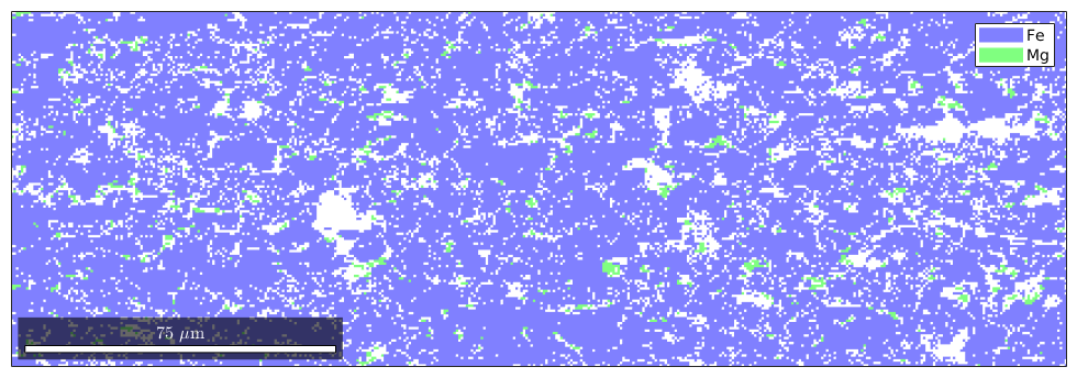
Plot Spatial Data

plot(ebsd)

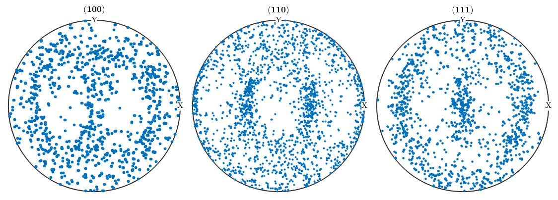
Plot Pole Figures as Scatter Plots

h = [Miller(1,0,0,CS{2}),Miller(1,1,0,CS{2}),Miller(1,1,1,CS{2})];

plotPDF(ebsd('Fe').orientations,h,'points',500,'antipodal')

  I'm plotting 500 random orientations out of 48184 given orientations
  You can specify the the number points by the option "points".
  The option "all" ensures that all data are plotted

Kernel Density Estimation

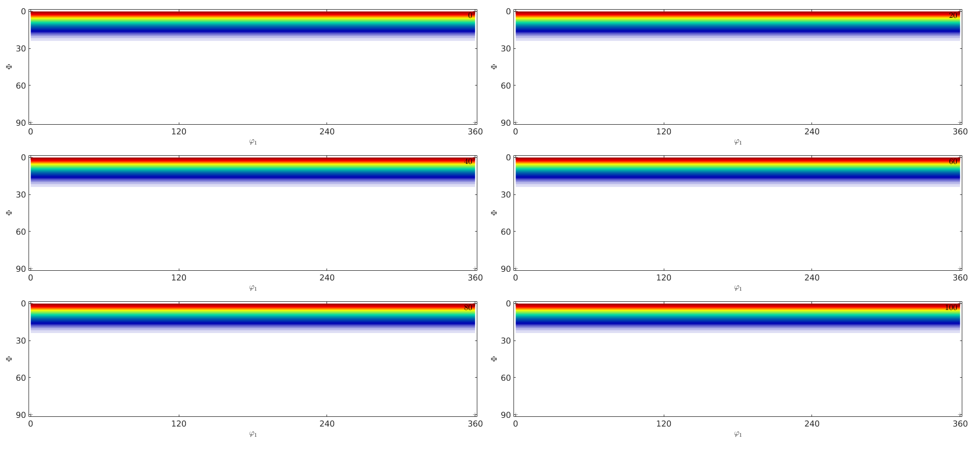
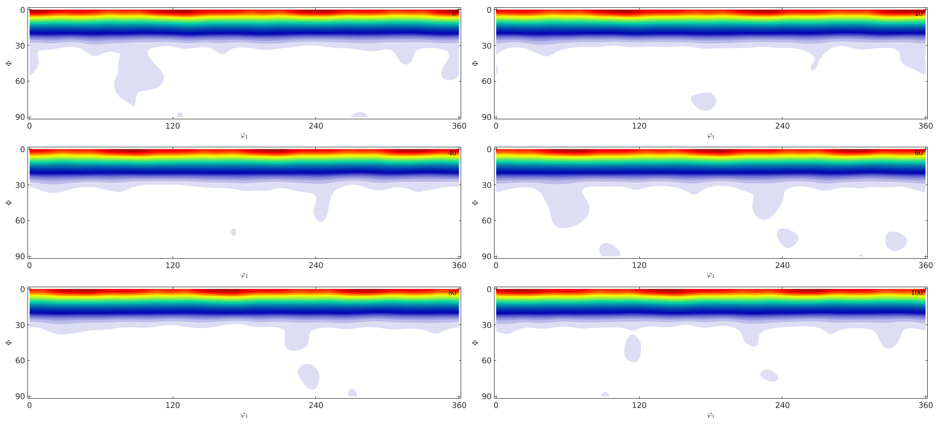
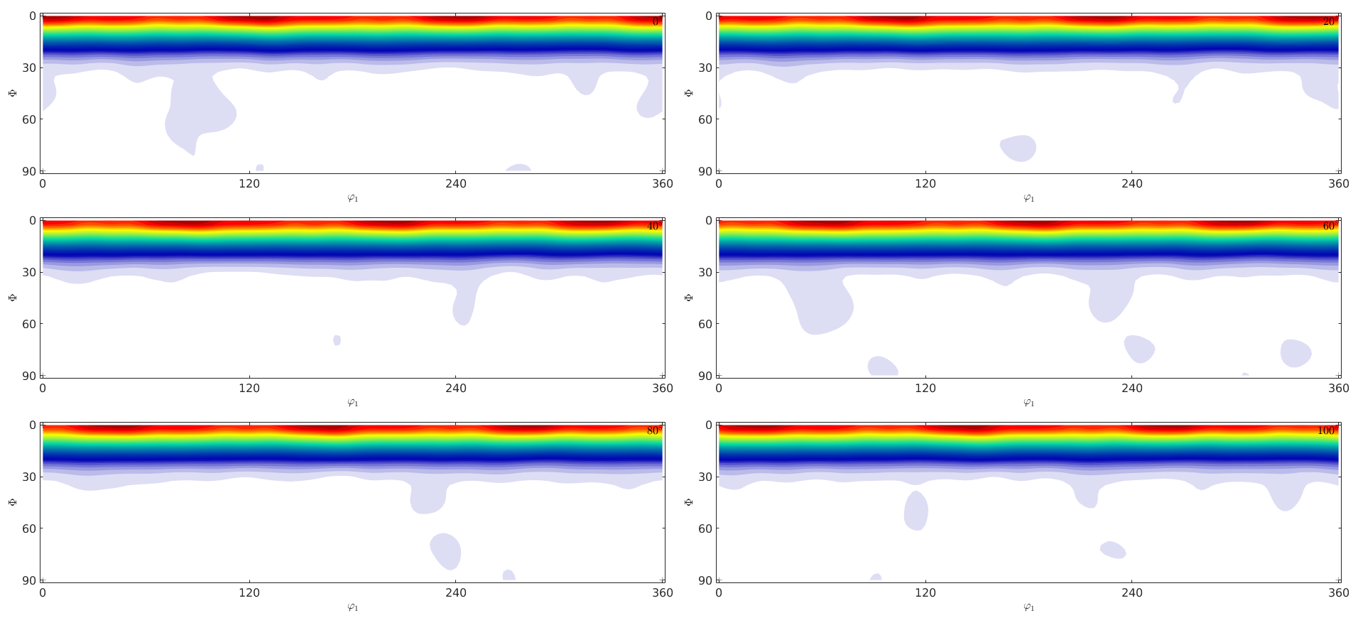
The crucial point in kernel density estimation in the choice of the halfwidth of the kernel function used for estimation. If the halfwidth of is chosen to small the single orientations are visible rather then the ODF (compare plot of ODF1). If the halfwidth is chosen to wide the estimated ODF becomes very smooth (ODF2).

odf1 = calcODF(ebsd('Fe').orientations)
odf2 = calcODF(ebsd('Fe').orientations,'halfwidth',5*degree)

 
odf1 = ODF  
  crystal symmetry : Fe (m-3m)
  specimen symmetry: 1
 
  Harmonic portion:
    degree: 25
    weight: 1
 
 
odf2 = ODF  
  crystal symmetry : Fe (m-3m)
  specimen symmetry: 1
 
  Harmonic portion:
    degree: 48
    weight: 1

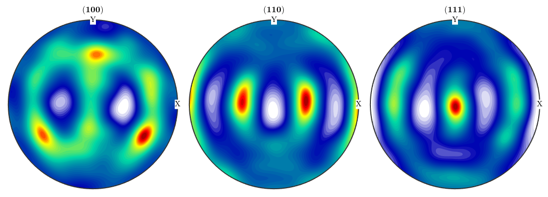
Plot pole figures

plotPDF(odf1,h,'antipodal')
figure
plotPDF(odf2,h,'antipodal')

Plot ODF

plot(odf2,'sections',9,'resolution',2*degree,...
  'FontSize',10,'silent')

Warning: Plot properties not compatible to previous plot! I'going to create a
new figure.

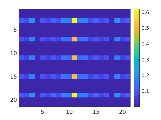
Estimation of Fourier Coefficients

Once, a ODF has been estimated from EBSD data it is straight forward to calculate Fourier coefficients. E.g. by

close all
odf2 = FourierODF(odf2);
imagesc(abs(odf2.calcFourier('order',10)))
mtexColorbar

However this is a biased estimator of the Fourier coefficents which underestimates the true Fourier coefficients by a factor that correspondes to the decay rate of the Fourier coeffients of the kernel used for ODF estimation. One obtains an unbiased estimator of the Fourier coefficients if they are calculated from the ODF estimated with the help fo the Direchlet kernel. I.e.

dirichlet = DirichletKernel(32);
odf3 = calcODF(ebsd('Fe').orientations,'kernel',dirichlet);
imagesc(abs(odf3.calcFourier('order',10)))
mtexColorbar

Let us compare the Fourier coefficients obtained by both methods.

plotFourier(odf2,'bandwidth',32)
hold all
plotFourier(odf3,'bandwidth',32)
hold off

A Sythetic Example

Simulate EBSD data from a given standard ODF

CS = crystalSymmetry('trigonal');
fibre_odf = 0.5*uniformODF(CS) + 0.5*fibreODF(Miller(0,0,0,1,CS),zvector);
plot(fibre_odf,'sections',6,'silent')
ori = calcOrientations(fibre_odf,10000)

Warning: Plot properties not compatible to previous plot! I'going to create a
new figure. 
 
ori = orientation  
  size: 10000 x 1
  crystal symmetry : -31m, X||a*, Y||b, Z||c*
  specimen symmetry: 1

Estimate an ODF from the simulated EBSD data

odf = calcODF(ori)

 
odf = ODF  
  crystal symmetry : -31m, X||a*, Y||b, Z||c*
  specimen symmetry: 1
 
  Harmonic portion:
    degree: 25
    weight: 1

plot the estimated ODF

plot(odf,'sections',6,'silent')

Warning: Plot properties not compatible to previous plot! I'going to create a
new figure.

calculate estimation error

calcError(odf,fibre_odf,'resolution',5*degree)

ans =
    0.0945

For a more exhausive example see the EBSD Simulation demo!

Exercises

a) Load the EBSD data: data/ebsd\_txt/85\_829grad\_07\_09\_06.txt!

import_wizard('ebsd')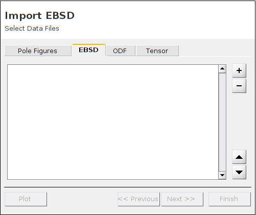

b) Estimate an ODF from the above EBSD data.

odf = calcODF(ori)

 
odf = ODF  
  crystal symmetry : -31m, X||a*, Y||b, Z||c*
  specimen symmetry: 1
 
  Harmonic portion:
    degree: 25
    weight: 1

c) Visualize the ODF and some of its pole figures!

plot(odf,'sections',6,'silent')

Warning: Plot properties not compatible to previous plot! I'going to create a
new figure.

d) Explore the influence of the halfwidth to the kernel density estimation by looking at the pole figures!